Abstract
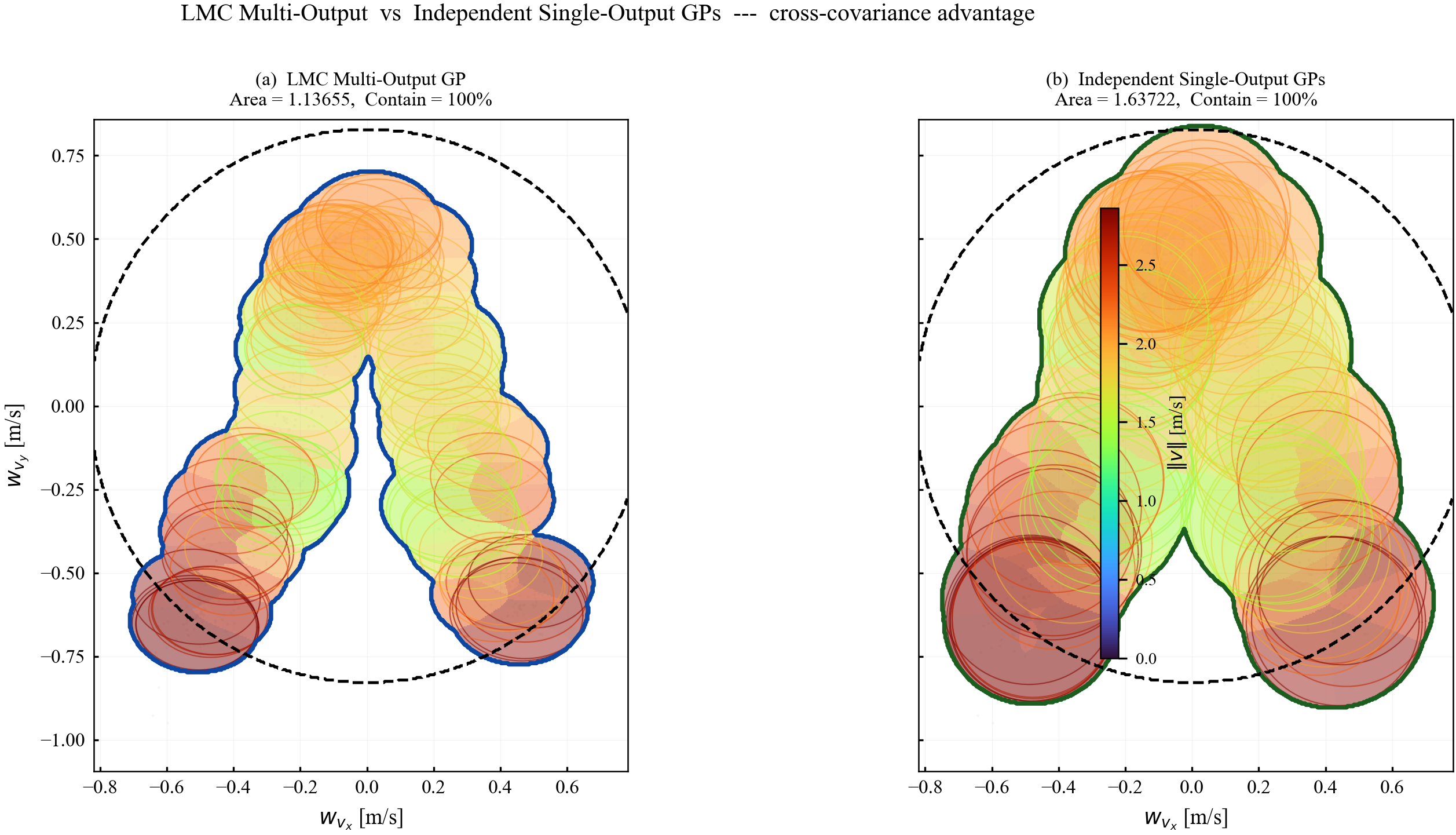
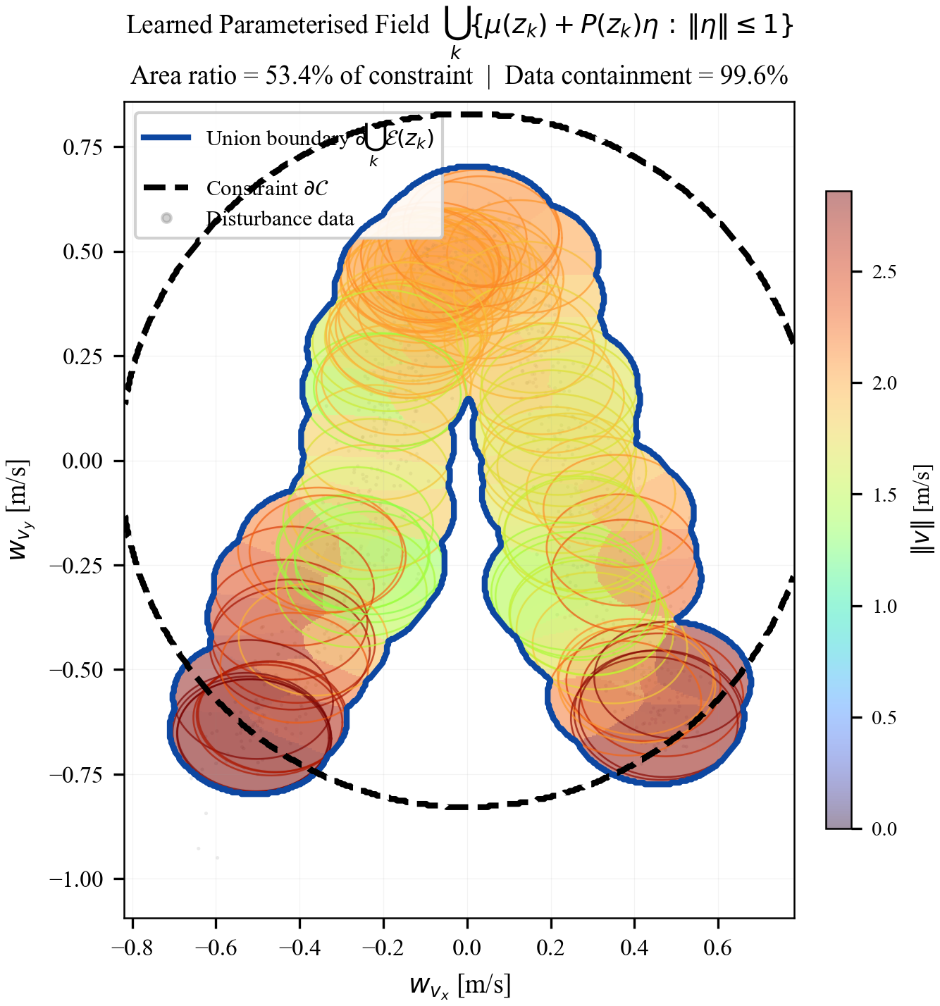
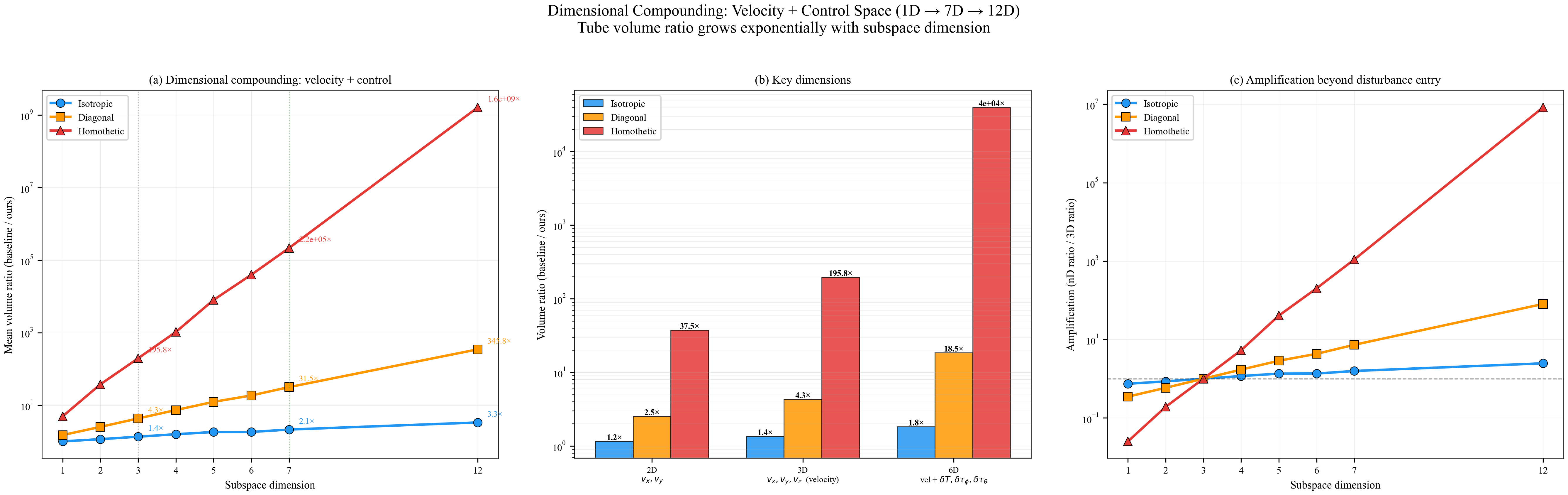
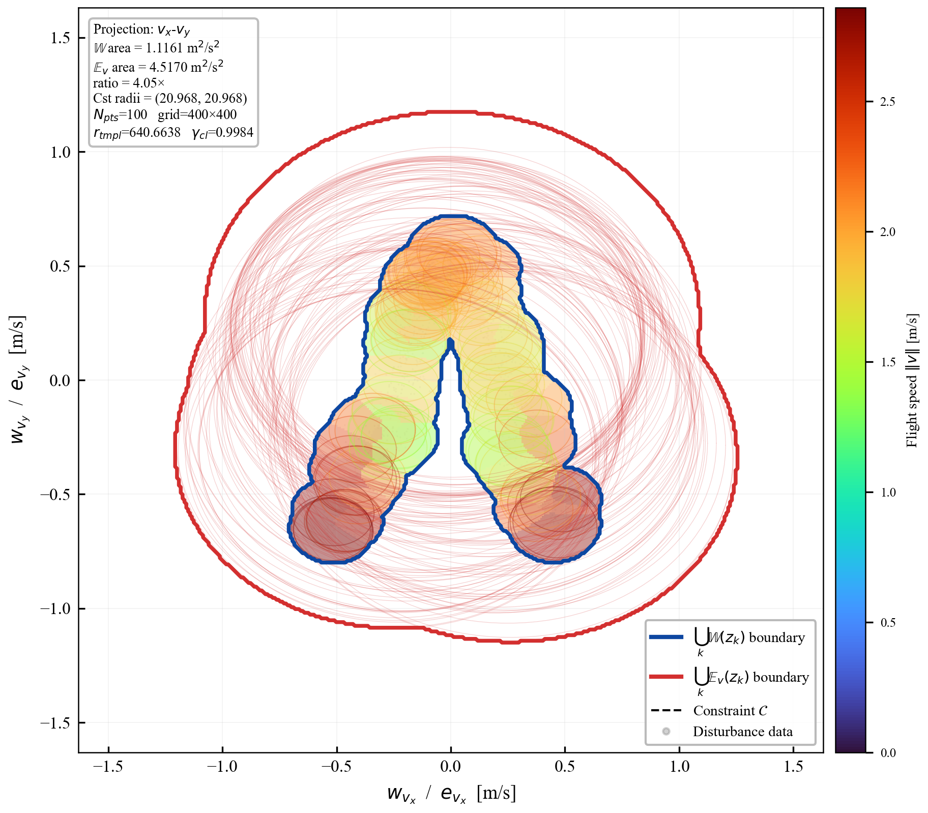
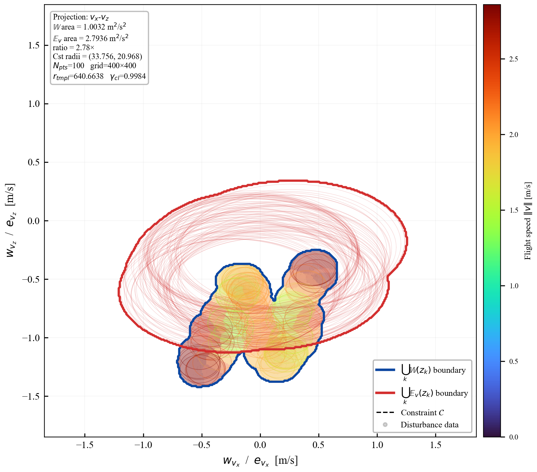
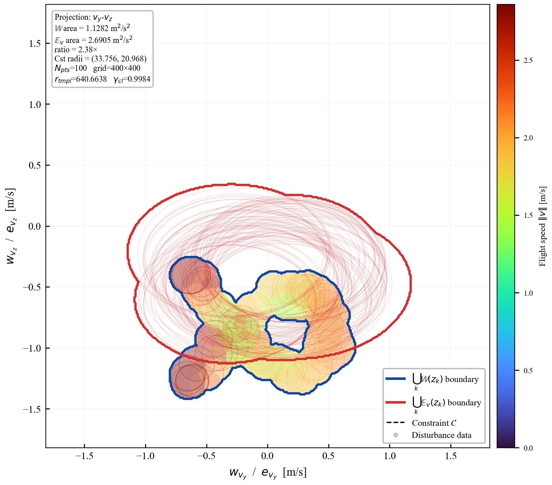
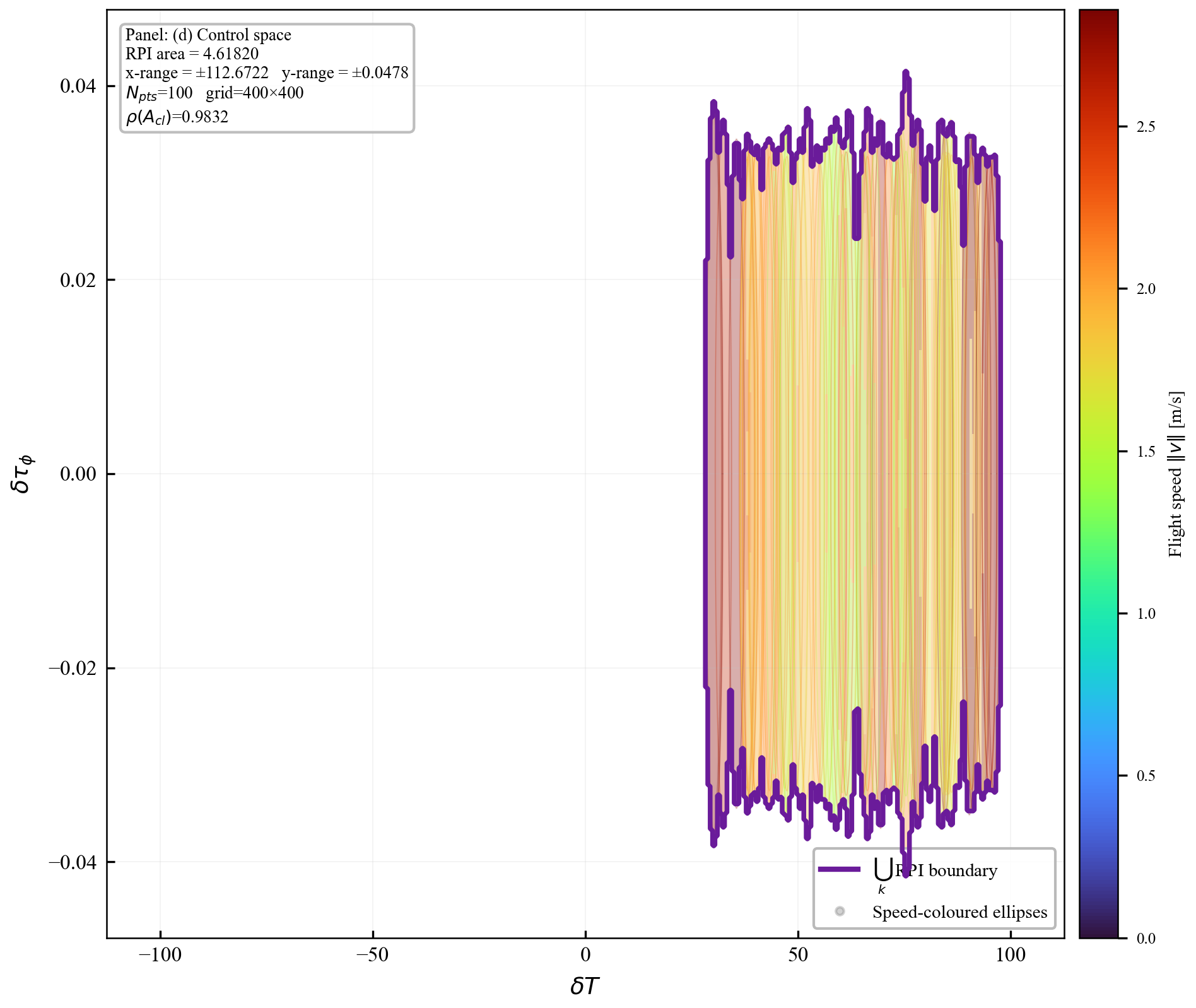
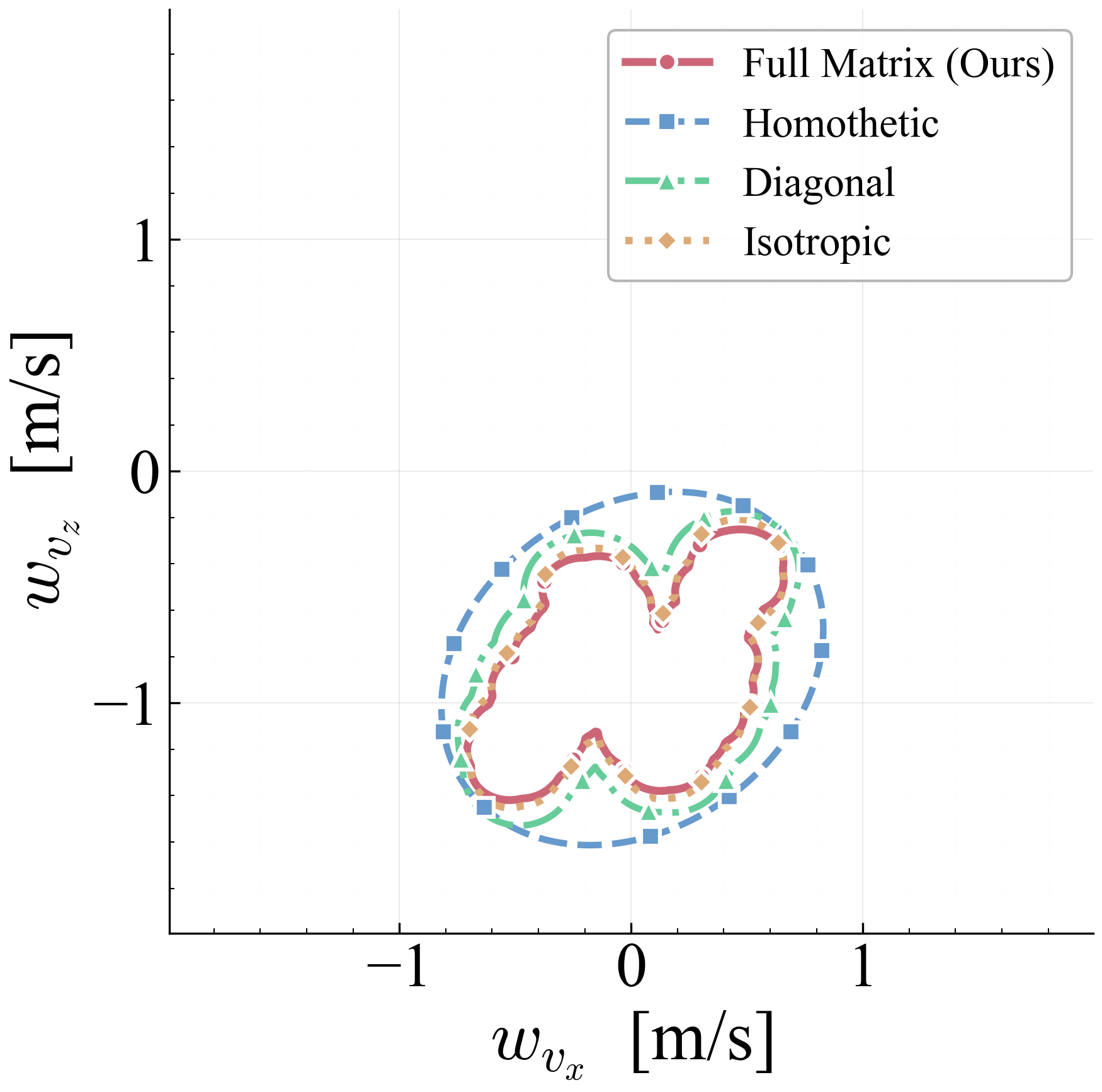
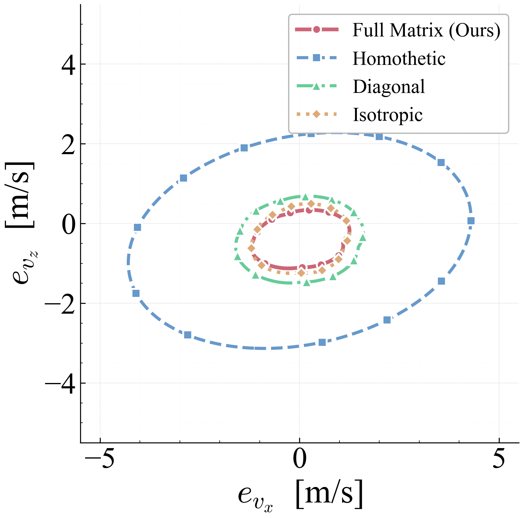
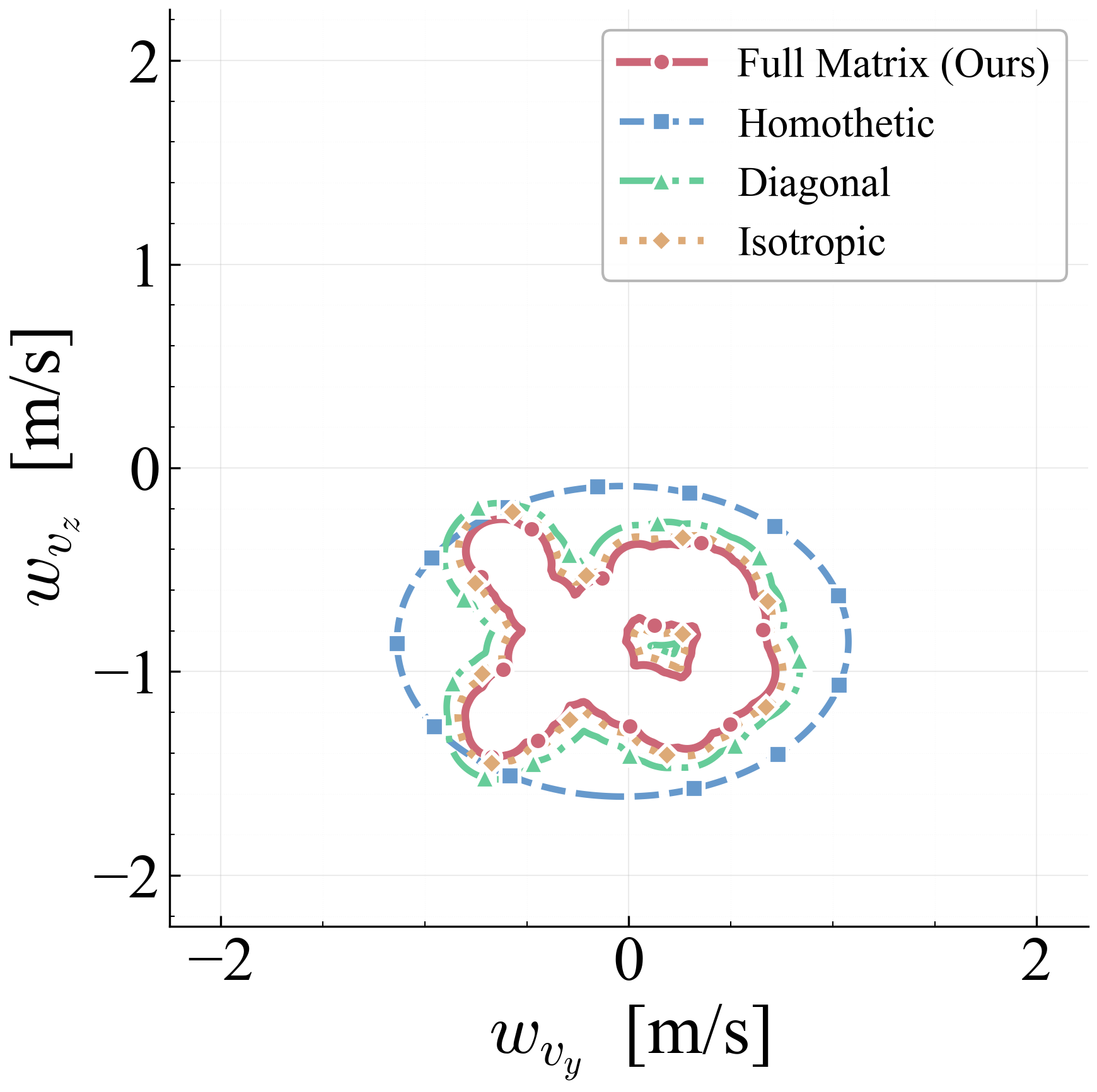
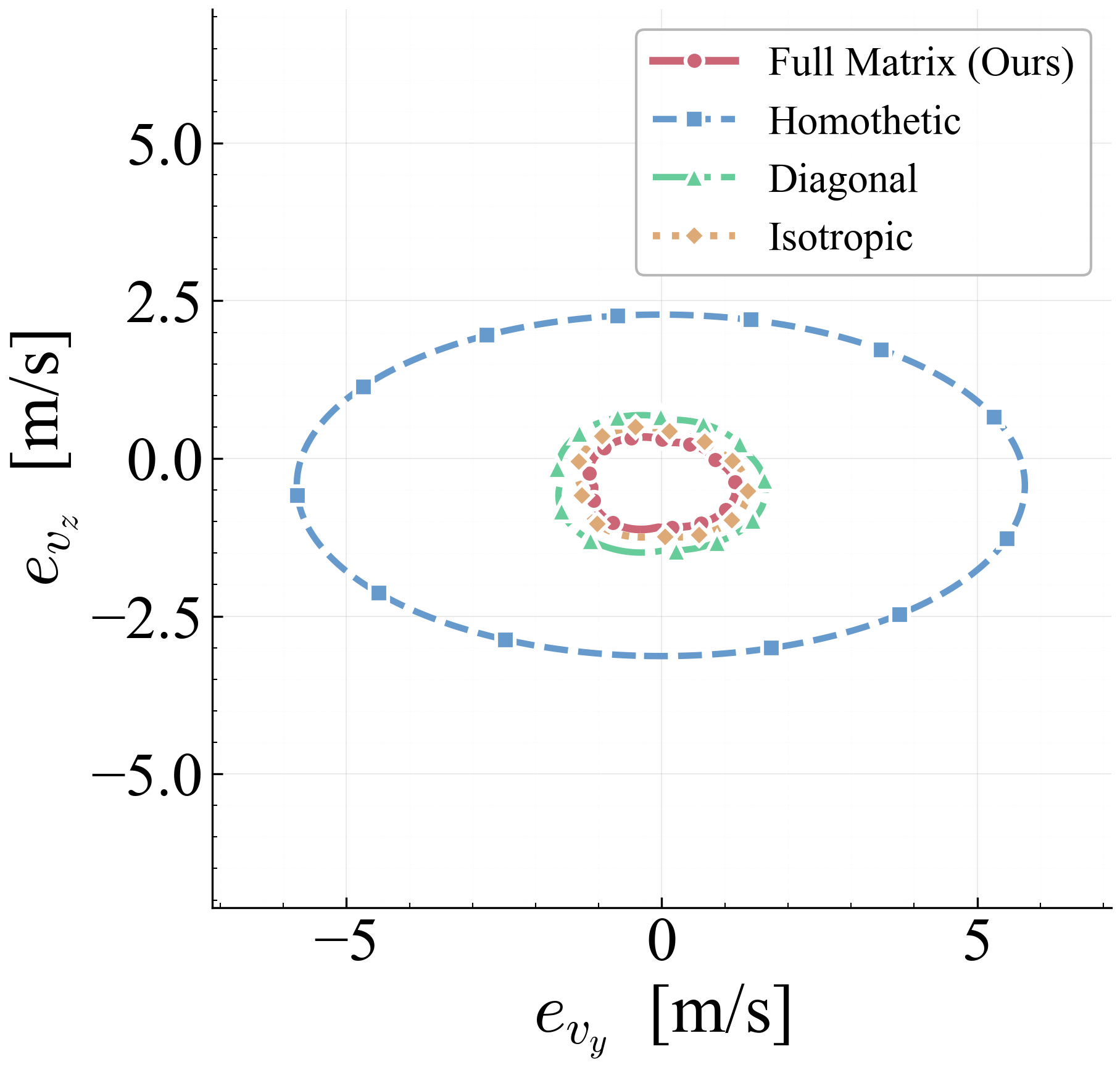
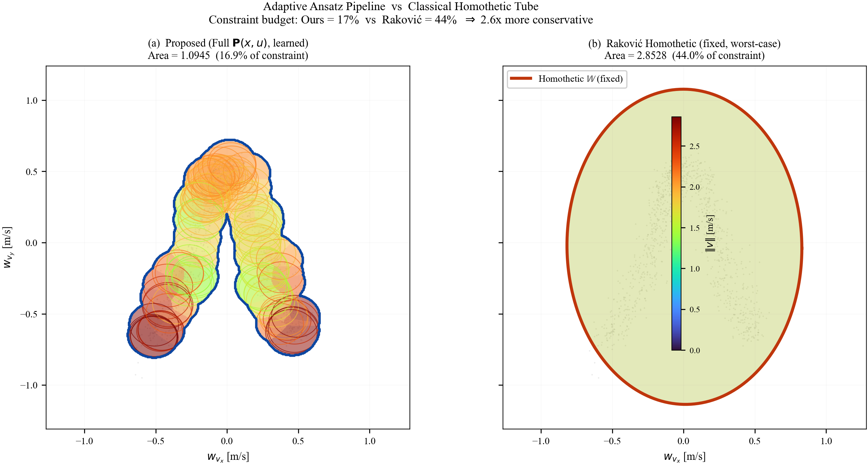
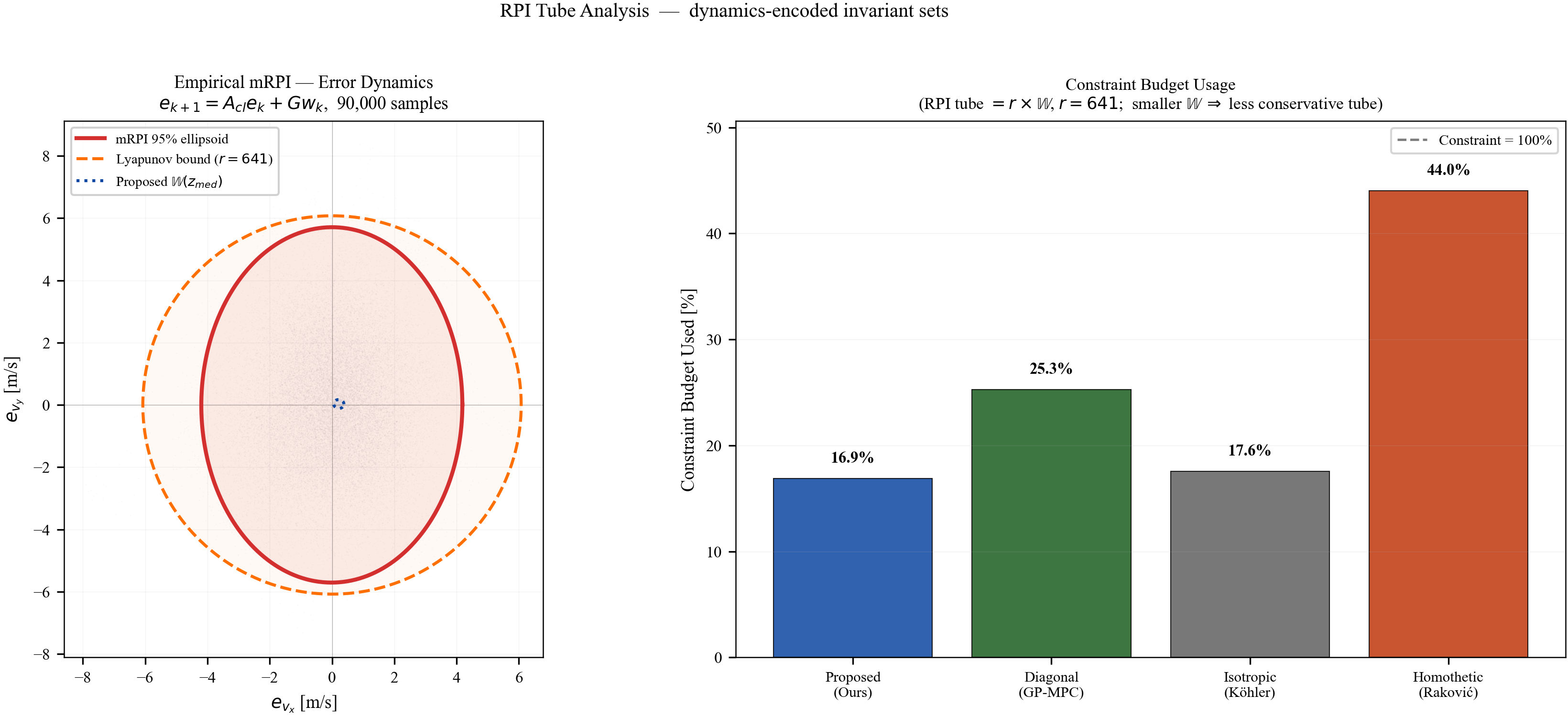
We establish sufficient conditions for robust positive invariance under state- and input-dependent disturbances with anisotropic covariance structure. The proposed ansätze map a fixed ellipsoidal template through a GP-derived positive-definite matrix field, subsuming scalar homothetic scaling while retaining finite graph-based verification. The resulting LMI conditions couple the learned field to Schur-stable dynamics; an isotropic fallback with inflation factor $r=1/(1-\gamma_{\mathrm{cl}})$ proves admissibility. During each learning epoch the field is frozen, so online tube evaluation is one GP covariance query and a small matrix square root, with no online set iteration or LMI solve. Quadrotor simulations show a $195\times$ reduction in 3D velocity-tube volume and a $2.1{\times}10^5$ reduction in the joint 7D velocity-control subspace relative to a non-adaptive homothetic baseline. This companion document expands the derivations behind the extended manuscript, including proof sketches, intuition boxes, controller-sweep figures, contraction studies, and projection-area comparisons.
Sets & Spaces
Symbol
Definition
Significance
$\mathbb{R}^n$, $\mathbb{R}^m$
Euclidean spaces of dimension $n$ (states) and $m$ (inputs)
Robust Model Predictive Control (MPC) requires disturbance-invariant sets for constraint satisfaction under uncertainty. The standard formulation assumes a fixed, state-independent disturbance set $\mathbb{W}\subset\mathbb{R}^n$ and computes a Robust Positively Invariant (RPI) set $\boldsymbol{\Omega}$ satisfying $\mathbf{A}_{\mathrm{cl}}\boldsymbol{\Omega}\oplus\mathbb{W}\subseteq\boldsymbol{\Omega}$. This is computationally tractable but conservative: a single $\mathbb{W}$ must bound worst-case disturbances uniformly, so spatial variation in uncertainty magnitude and orientation is lost.
Minkowski Sum. Given two sets $A,B\subset\mathbb{R}^n$, the Minkowski sum is $A\oplus B:=\{a+b: a\in A,\;b\in B\}$. Geometrically, it "inflates" $A$ by the shape of $B$.
Pontryagin Difference. The Pontryagin difference (or erosion) is $A\ominus B:=\{x\in\mathbb{R}^n: x+B\subseteq A\}$. It "shrinks" $A$ by $B$. Key property: $A\ominus B \subseteq A$ whenever $\mathbf{0}\in B$.
RPI connection. A set $\boldsymbol{\Omega}$ is RPI for $(\mathbf{A}_{\mathrm{cl}},\mathbb{W})$ when $\mathbf{A}_{\mathrm{cl}}\boldsymbol{\Omega}\oplus\mathbb{W}\subseteq\boldsymbol{\Omega}$, meaning at every point the "pushed-forward" set plus the disturbance set stays within $\boldsymbol{\Omega}$. Equivalently, $\mathbf{A}_{\mathrm{cl}}\boldsymbol{\Omega}\subseteq\boldsymbol{\Omega}\ominus\mathbb{W}$.
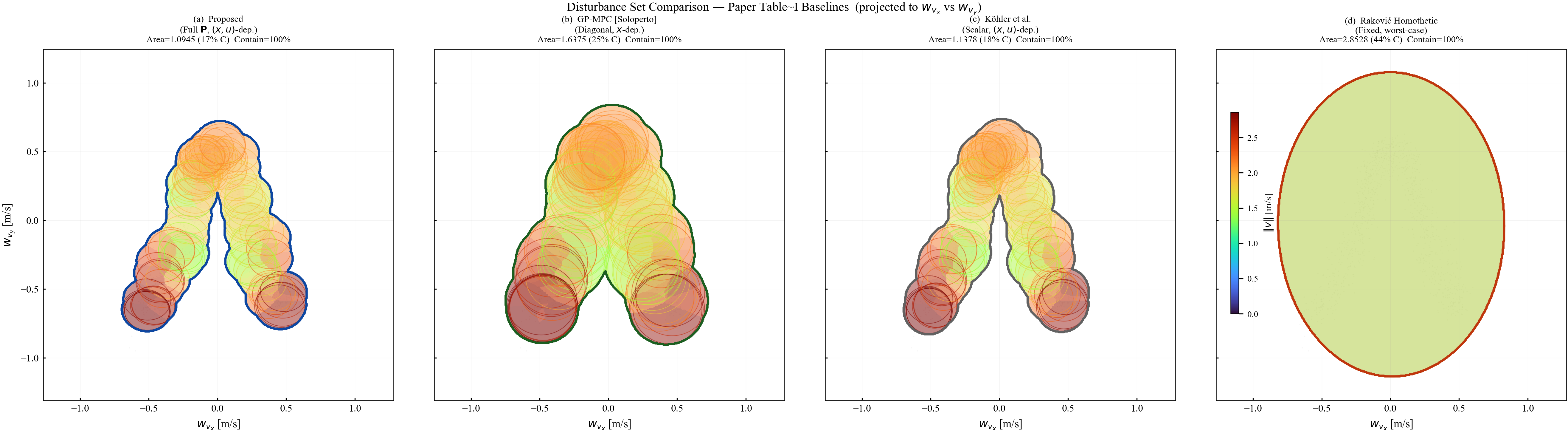
We observe that methods addressing this conservatism share a common structure: parameterization of disturbance or tube sets as transformations of a fixed template shape. We formalize this as a template ansatz, a structured trial form wherein $(\mathbf{x},\mathbf{u})$-dependence is encoded in transformation parameters rather than set geometry.
Scalar ansätze. Homothetic tube MPC uses $\alpha_k\bar{\boldsymbol{\Omega}}$ with scalar $\alpha_k$ optimized over the prediction horizon. Extensions learn stage-indexed scalars through Lipschitz analysis or the scenario approach. These methods capture magnitude variation but not directional structure.
Per-facet and shape-free ansätze. Elastic tubes generalize to per-facet scaling $\boldsymbol{\gamma}_k\in\mathbb{R}^p$, and configuration-constrained tubes optimize polytope vertices online. These permit richer geometric variation but remain stage-indexed: adaptation tracks the nominal trajectory rather than the current operating point.
Diagonal ansätze. GP-based methods construct confidence regions from posteriors, producing axis-aligned hyperboxes $\mathbb{W}(\mathbf{x})=\{\mathbf{w}:|w_j|\le\beta\sigma_{n,j}(\mathbf{x})\}$, equivalent to $\mathbf{P}=\mathrm{diag}(\sigma_1,\ldots,\sigma_n)$, but cannot represent inter-component correlations.
The gap. No existing method provides a full matrix $\mathbf{P}(\mathbf{x},\mathbf{u})\in\mathbb{S}^n_{++}$ that varies with the current operating point and is learned from data.
Table I: Template ansätze in the literature and the proposed generalization.
Method
Transformation
Depends on
Learned
Homothetic
Scalar $\alpha$
Stage $k$
No
Elastic
Per-facet $\boldsymbol{\gamma}$
Stage $k$
No
CCTMPC
Full shape
Stage $k$
No
Kohler et al.
Scalar
$(\mathbf{x},\mathbf{u})$
No
GP-MPC
Diagonal
$\mathbf{x}$ only
Yes
Scenario
Scalar
Stage $k$
Yes
Proposed
Full matrix $\mathbf{P}$
$(\mathbf{x},\mathbf{u})$
Yes
Relation to prior work. State- and input-dependent disturbances induce a circular dependence: verifying that states remain within a candidate invariant set requires knowledge of reachable states, which depends on the invariant set. Our prior work resolves this by lifting the dynamics to an augmented space $\mathbb{R}^{2n+m}$, where the disturbance law becomes a graph constraint, and then computing RPI sets as fixed points of a set-valued operator. That lifted fixed-point method is exact but computationally expensive: polytope iterations require seconds with GPU acceleration and can take minutes without it. The present work takes a different route. The base template pair $(\bar{\mathbf{W}}, \bar{\boldsymbol{\Omega}})$ is computed once at initialization; thereafter, invariance is enforced by constraining the parameter field $\mathbf{P}(\cdot)$ rather than by recomputing set geometry.
Richer transformation classes. The template ansatz framework naturally suggests a hierarchy of increasing expressiveness: scalar (homothetic), diagonal, symmetric positive-definite (present work), general linear, and polynomial. The latter would parameterize disturbance sets as semialgebraic sublevel sets $\mathbb{W} = \{\mathbf{w} : p(\mathbf{w}; \mathbf{x}, \mathbf{u}) \leq 1\}$ with verification via sum-of-squares programming. This could capture non-ellipsoidal uncertainty structure at higher computational cost.
Contributions. We introduce the anisotropic template ansatz
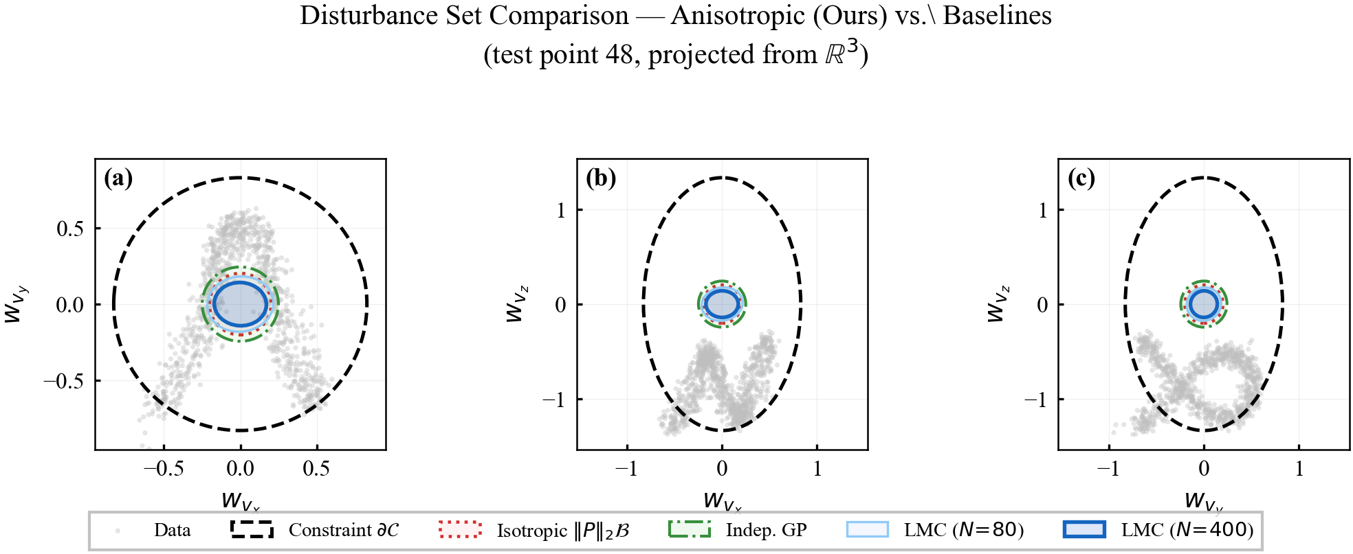
where $\bar{\mathbf{W}}\subset\mathbb{R}^n$ is a fixed template and $\mathbf{P}(\mathbf{x},\mathbf{u})\in\mathbb{S}^n_{++}$ encodes local anisotropy learned from GP posteriors via $\mathbf{P}=c_{n,\alpha}\hat{\boldsymbol{\Sigma}}_w^{1/2}$.
Template ansatz formalism. Unification of scalar, diagonal, and full-matrix parameterizations under a single framework indexed by transformation class.
Parameter-space invariance conditions. Sufficient conditions for RPI formulated as LMIs coupling $\mathbf{P}(\cdot)$ to closed-loop dynamics, bypassing set-valued iteration.
Graph-based finite verification. Discretization of the continuous operating space into a finite graph with arc-wise spectral conditions.
Single-query online evaluation. After offline GP training and graph verification, each online tube cross-section is obtained by one GP covariance query and one small matrix square root, independent of horizon length, graph size, and iteration count. The base template pair $(\bar{\mathbf{W}}, \bar{\boldsymbol{\Omega}})$ is fixed after initialization; subsequent learning epochs refine only $\mathbf{P}^{(q)}(\cdot)$, and tubes contract monotonically as data accumulate.
II. Anisotropic Template Geometry
Consider a discrete-time system with nominal linear dynamics and additive state- and input-dependent uncertainty:
where $\mathbf{x}_k\in\mathcal{X}\subseteq\mathbb{R}^n$, $\mathbf{u}_k\in\mathcal{U}\subseteq\mathbb{R}^m$, $(\mathbf{A},\mathbf{B})$ are nominal matrices, and $\mathbf{w}(\mathbf{x},\mathbf{u})\in\mathbb{W}(\mathbf{x},\mathbf{u})\subset\mathbb{R}^n$ is a state- and input-dependent residual. Thus $\mathbf{A},\mathbf{B}$ are assumed available from modeling, local linearization, or identification; in the latter case $\mathbf{w}$ also absorbs identification error.
A matrix $\mathbf{A}\in\mathbb{R}^{n\times n}$ is Schur stable if all its eigenvalues lie strictly inside the unit circle: $\rho(\mathbf{A}):=\max_i|\lambda_i(\mathbf{A})|<1$. The number $\rho(\mathbf{A})$ is the spectral radius.
Why it matters here. For the error dynamics $\mathbf{e}_{k+1}=\mathbf{A}_{\mathrm{cl}}\mathbf{e}_k+\mathbf{w}_k$, Schur stability of $\mathbf{A}_{\mathrm{cl}}$ ensures that disturbance effects do not accumulate unboundedly. Without it, no bounded invariant set can exist (the error can grow arbitrarily). With $\rho(\mathbf{A}_{\mathrm{cl}})<1$, the "contraction" from $\mathbf{A}_{\mathrm{cl}}$ can compensate for the "expansion" from $\mathbf{w}_k$, enabling bounded tubes.
Discrete vs. continuous. In continuous time the analogous concept is Hurwitz stability (eigenvalues in the open left half-plane). In discrete time we use Schur stability (eigenvalues inside the unit disk).
Assumption 1 (Standing Hypotheses)
The constraint sets $\mathcal{X}$, $\mathcal{U}$ are compact and convex. A stabilizing gain $\mathbf{K}\in\mathbb{R}^{m\times n}$ exists such that $\mathbf{A}_{\mathrm{cl}}:=\mathbf{A}+\mathbf{B}\mathbf{K}$ is Schur stable, i.e., $\rho(\mathbf{A}_{\mathrm{cl}})<1$.
Under affine feedback $\mathbf{u}=\mathbf{K}\mathbf{x}+\mathbf{v}$, the error $\mathbf{e}_k:=\mathbf{x}_k-\hat{\mathbf{x}}_k$ relative to a nominal trajectory satisfies
An anisotropic template ansatz is a family $\mathbb{W}(\mathbf{x},\mathbf{u})=\mathbf{P}(\mathbf{x},\mathbf{u})\bar{\mathbf{W}}:=\{\mathbf{P}(\mathbf{x},\mathbf{u})\mathbf{w}:\mathbf{w}\in\bar{\mathbf{W}}\}$ where $\bar{\mathbf{W}}\subset\mathbb{R}^n$ is a fixed template with $\mathbf{0}\in\mathrm{int}(\bar{\mathbf{W}})$ and $\mathbf{P}:\mathcal{X}\times\mathcal{U}\to\mathbb{S}^n_{++}$ maps to the cone of symmetric positive-definite matrices.
A symmetric matrix $\mathbf{P}\in\mathbb{R}^{n\times n}$ (i.e., $\mathbf{P}=\mathbf{P}^\top$) belongs to $\mathbb{S}^n_{++}$ (positive definite) if $\mathbf{v}^\top\mathbf{P}\mathbf{v}>0$ for all nonzero $\mathbf{v}\in\mathbb{R}^n$, and to $\mathbb{S}^n_+$ (positive semidefinite) if $\mathbf{v}^\top\mathbf{P}\mathbf{v}\ge 0$.
Spectral decomposition. Any symmetric $\mathbf{P}$ admits the decomposition $\mathbf{P}=\mathbf{V}\boldsymbol{\Lambda}\mathbf{V}^\top$ where $\mathbf{V}$ is orthogonal (columns are eigenvectors) and $\boldsymbol{\Lambda}=\mathrm{diag}(\lambda_1,\ldots,\lambda_n)$ are the eigenvalues. The matrix is positive definite iff all $\lambda_i>0$.
Geometric meaning. The set $\mathbf{P}\mathcal{B}_2^n$ (image of the unit ball under $\mathbf{P}$) is an ellipsoid whose principal axes have directions $\mathbf{v}_i$ and lengths $\lambda_i$. The matrix $\mathbf{P}$ thus encodes both orientation and shape of this ellipsoid, which is why it captures anisotropic (direction-dependent) uncertainty.
Matrix square root. If $\mathbf{P}\in\mathbb{S}^n_{++}$, there exists a unique $\mathbf{P}^{1/2}\in\mathbb{S}^n_{++}$ such that $(\mathbf{P}^{1/2})^2=\mathbf{P}$. Via the spectral decomposition: $\mathbf{P}^{1/2}=\mathbf{V}\boldsymbol{\Lambda}^{1/2}\mathbf{V}^\top$.
The matrix $\mathbf{P}(\mathbf{x},\mathbf{u})$ encodes local anisotropy via its spectral decomposition: eigenvectors define principal uncertainty directions; eigenvalues set magnitudes along these axes. Setting $\mathbf{P}=\sigma\mathbf{I}_n$ recovers isotropic scaling; $\mathbf{P}=\mathrm{diag}(\sigma_1,\ldots,\sigma_n)$ yields axis-aligned boxes; the general case admits rotation and shear.
GP Posteriors as Anisotropy Fields
From trajectory data, disturbance samples $\mathbf{w}^{(j)}=\mathbf{x}^{(j+1)}-\mathbf{A}\mathbf{x}^{(j)}-\mathbf{B}\mathbf{u}^{(j)}$ yield dataset $\mathcal{D}=\{(\mathbf{z}^{(j)},\mathbf{w}^{(j)})\}_{j=1}^N$ with $\mathbf{z}:=(\mathbf{x},\mathbf{u})\in\mathcal{Z}:=\mathcal{X}\times\mathcal{U}$. The GP posterior covariance $\hat{\boldsymbol{\Sigma}}_w(\mathbf{x},\mathbf{u})\in\mathbb{S}^n_+$ yields the $(1-\alpha)$ credible region:
where $c_{n,\alpha}:=\sqrt{\chi^2_{n,1-\alpha}}$ and $\mathcal{B}_2^n$ is the Euclidean unit ball. The GP-induced anisotropy field is $\mathbf{P}(\mathbf{x},\mathbf{u}):=c_{n,\alpha}\hat{\boldsymbol{\Sigma}}_w(\mathbf{x},\mathbf{u})^{1/2}$.
Base Template and Invariance Geometry
The base template pair $(\bar{\mathbf{W}},\bar{\boldsymbol{\Omega}})$ is computed once at initialization. We fix $\bar{\mathbf{W}} = \mathcal{B}_2^n$ and set the tube template to $\bar{\boldsymbol{\Omega}} = r\mathcal{B}_2^n$, with template inflation factor
$$r \;:=\; \frac{1}{1 - \gamma_{\mathrm{cl}}}.$$
Here the closed-loop contraction rate $\gamma_{\mathrm{cl}} < 1$ is defined as follows: if $\|\mathbf{A}_{\mathrm{cl}}\|_2 < 1$ set $\gamma_{\mathrm{cl}} := \|\mathbf{A}_{\mathrm{cl}}\|_2$; otherwise set $\gamma_{\mathrm{cl}} := \sqrt{\rho(\mathbf{P}_{\mathrm{d}}^{-1}\mathbf{A}_{\mathrm{cl}}^\top\mathbf{P}_{\mathrm{d}}\,\mathbf{A}_{\mathrm{cl}})}$ where $\mathbf{P}_{\mathrm{d}} \succ \mathbf{0}$ is the DARE terminal-cost matrix. Schur stability guarantees $\gamma_{\mathrm{cl}} < 1$ in both cases.
The template inflation factor $r$ is the minimal scalar ensuring $\gamma_{\mathrm{cl}}\,r + 1 \leq r$, i.e., $r\mathcal{B}_2^n$ is RPI for $(\mathbf{A}_{\mathrm{cl}}, \mathcal{B}_2^n)$. The tube template $\bar{\boldsymbol{\Omega}}$ is strictly larger than $\bar{\mathbf{W}}$; this separation provides the geometric headroom that makes the invariance conditions feasible. Subsequent analysis constrains only $\mathbf{P}(\cdot)$.
Remark (Lyapunov Coordinate Change)
When $\|\mathbf{A}_{\mathrm{cl}}\|_2 < 1$, one sets $\mathbf{P}_{\mathrm{d}} = \mathbf{I}_n$ and $\gamma_{\mathrm{cl}} = \|\mathbf{A}_{\mathrm{cl}}\|_2$. When $\|\mathbf{A}_{\mathrm{cl}}\|_2 \geq 1$ (e.g. a 12-state quadrotor with $\rho(\mathbf{A}_{\mathrm{cl}}) < 1$), the change of coordinates $\tilde{\mathbf{e}} = \mathbf{P}_{\mathrm{d}}^{1/2}\mathbf{e}$ yields $\|\tilde{\mathbf{A}}_{\mathrm{cl}}\|_2 = \gamma_{\mathrm{cl}} < 1$, reducing to the same framework. All spectral conditions in Sections III–IV use $\gamma_{\mathrm{cl}}$ accordingly, with spectral bounds $p_i^{\pm}$ understood in the $\mathbf{P}_{\mathrm{d}}$-weighted norm.
Assumption 2 (Anisotropy Field Regularity)
The map $\mathbf{P}:\mathcal{Z}\to\mathbb{S}^n_{++}$ satisfies uniform Löwner bounds $p_{\min}\mathbf{I}_n\preceq\mathbf{P}(\mathbf{z})\preceq p_{\max}\mathbf{I}_n$ with $0\lt p_{\min}\le p_{\max}\lt\infty$, and is Lipschitz continuous with constant $L_P\gt 0$.
Local RPI Fields and the Invariance Problem
For a compact convex set $\mathbf{S}\subset\mathbb{R}^n$ with $\mathbf{0}\in\mathrm{int}(\mathbf{S})$, the gauge function is
It measures "how far" $\mathbf{w}$ is from the origin relative to $\mathbf{S}$: $\gamma_{\mathbf{S}}(\mathbf{w})\le 1$ iff $\mathbf{w}\in\mathbf{S}$; $\gamma_{\mathbf{S}}(\mathbf{w})=2$ means $\mathbf{w}$ is twice as far as the boundary of $\mathbf{S}$.
Properties: (i) $\gamma_{\mathbf{S}}(\alpha\mathbf{w})=\alpha\,\gamma_{\mathbf{S}}(\mathbf{w})$ for $\alpha\ge 0$ (positive homogeneity); (ii) $\gamma_{\mathbf{S}}(\mathbf{w}_1+\mathbf{w}_2)\le\gamma_{\mathbf{S}}(\mathbf{w}_1)+\gamma_{\mathbf{S}}(\mathbf{w}_2)$ (subadditivity); (iii) for invertible $\mathbf{M}$: $\gamma_{\mathbf{M}\mathbf{S}}(\mathbf{w})=\gamma_{\mathbf{S}}(\mathbf{M}^{-1}\mathbf{w})$.
Special case. For the unit ball $\mathcal{B}_2^n$, the gauge is the Euclidean norm: $\gamma_{\mathcal{B}_2^n}(\mathbf{w})=\|\mathbf{w}\|_2$. For the ellipsoid $\mathbf{P}\mathcal{B}_2^n$ with $\mathbf{P}\succ\mathbf{0}$: $\gamma_{\mathbf{P}\mathcal{B}_2^n}(\mathbf{w})=\|\mathbf{P}^{-1}\mathbf{w}\|_2$.
Definition 2 (Template Contraction Coefficient)
For Schur-stable $\mathbf{A}_{\mathrm{cl}}$ and template $\bar{\boldsymbol{\Omega}}\ni\mathbf{0}$, the contraction coefficient is $\rho_{\bar{\boldsymbol{\Omega}}}:=\sup_{\mathbf{e}\in\bar{\boldsymbol{\Omega}}}\gamma_{\bar{\boldsymbol{\Omega}}}(\mathbf{A}_{\mathrm{cl}}\mathbf{e})$.
Lemma 1 (Strict Contraction)
If $\bar{\boldsymbol{\Omega}}$ is RPI for $(\mathbf{A}_{\mathrm{cl}},\bar{\mathbf{W}})$ with $\mathbf{0}\in\mathrm{int}(\bar{\mathbf{W}})$, then $\rho_{\bar{\boldsymbol{\Omega}}}<1$.
Goal. Show that $\rho_{\bar{\boldsymbol{\Omega}}} := \sup_{\mathbf{e} \in \bar{\boldsymbol{\Omega}}} \gamma_{\bar{\boldsymbol{\Omega}}}(\mathbf{A}_{\mathrm{cl}} \mathbf{e}) < 1$.
Step 1 (RPI implies Pontryagin containment). By definition, $\bar{\boldsymbol{\Omega}}$ is RPI for $(\mathbf{A}_{\mathrm{cl}}, \bar{\mathbf{W}})$ means:
By the definition of the Pontryagin difference, $A \oplus B \subseteq C$ if and only if $A \subseteq C \ominus B$. Applying this with $A = \mathbf{A}_{\mathrm{cl}}\bar{\boldsymbol{\Omega}}$, $B = \bar{\mathbf{W}}$, $C = \bar{\boldsymbol{\Omega}}$:
Step 2 (Interior point implies strict erosion). Since $\mathbf{0} \in \mathrm{int}(\bar{\mathbf{W}})$, there exists $\varepsilon > 0$ such that $\varepsilon \mathcal{B}_2^n \subseteq \bar{\mathbf{W}}$. A classical result in set-valued analysis (see Blanchini, Proposition 3.2) states that for compact convex $\bar{\boldsymbol{\Omega}}$ and $\bar{\mathbf{W}}$ with $\mathbf{0} \in \mathrm{int}(\bar{\mathbf{W}})$:
for some $\delta > 0$. Intuitively, eroding $\bar{\boldsymbol{\Omega}}$ by a set with nonempty interior strictly shrinks it.
Step 3 (Derive the $\delta$ explicitly). To see why $\delta$ exists: for any $\mathbf{e} \in \bar{\boldsymbol{\Omega}} \ominus \bar{\mathbf{W}}$, we have $\mathbf{e} + \bar{\mathbf{W}} \subseteq \bar{\boldsymbol{\Omega}}$. In particular, $\mathbf{e} + \varepsilon \mathcal{B}_2^n \subseteq \bar{\boldsymbol{\Omega}}$, so $\mathbf{e}$ is at least distance $\varepsilon$ from the boundary of $\bar{\boldsymbol{\Omega}}$ (in the gauge metric). Since $\bar{\boldsymbol{\Omega}}$ is compact and contains the origin in its interior, let $R := \sup_{\mathbf{e} \in \bar{\boldsymbol{\Omega}}} \|\mathbf{e}\|_2$ be the circumradius. Then $\gamma_{\bar{\boldsymbol{\Omega}}}(\mathbf{e}) \le 1 - \varepsilon/R$ for all $\mathbf{e} \in \bar{\boldsymbol{\Omega}} \ominus \bar{\mathbf{W}}$. We may take $\delta = \varepsilon / R > 0$.
Step 4 (Chain the containments). Combining Steps 1 and 2:
Step 5 (Conclude via gauge function). For any $\mathbf{e} \in \bar{\boldsymbol{\Omega}}$, we have $\mathbf{A}_{\mathrm{cl}}\mathbf{e} \in (1 - \delta)\bar{\boldsymbol{\Omega}}$, which means $\gamma_{\bar{\boldsymbol{\Omega}}}(\mathbf{A}_{\mathrm{cl}}\mathbf{e}) \le 1 - \delta$. Taking the supremum over all $\mathbf{e} \in \bar{\boldsymbol{\Omega}}$:
A map $\mathbf{x}\mapsto\mathcal{B}(\mathbf{x})$ is a local RPI field if the graph $\mathcal{O}:=\bigcup_{\mathbf{x}\in\mathcal{X}}(\mathbf{x}+\mathcal{B}(\mathbf{x}))$ is RPI for the closed-loop system: $\mathbf{x}_k\in\mathcal{O}\Rightarrow\mathbf{x}_{k+1}\in\mathcal{O}$ for all admissible $\mathbf{w}_k\in\mathbb{W}(\mathbf{x}_k,\mathbf{u}_k)$.
Problem 1 (Anisotropic Template Invariance)
Given dynamics, template pair $(\bar{\mathbf{W}}, \bar{\boldsymbol{\Omega}}) = (\mathcal{B}_2^n, r\mathcal{B}_2^n)$ with $r = 1/(1-\gamma_{\mathrm{cl}})$, and GP-induced field $\mathbf{P}(\mathbf{x},\mathbf{u})$ satisfying Assumption 2, find conditions on $\mathbf{P}(\cdot)$ such that $\boldsymbol{\Omega}(\mathbf{x},\mathbf{u}):=\mathbf{P}(\mathbf{x},\mathbf{u})\bar{\boldsymbol{\Omega}}$ is a local RPI field.
III. Learning the Anisotropy Field from Data
This section constructs $\mathbf{P}(\mathbf{x},\mathbf{u})$ from trajectory data via Gaussian Process regression and establishes regularity properties required for invariance.
A Gaussian Process (GP) is a collection of random variables, any finite number of which have a joint Gaussian distribution. A GP is fully specified by a mean function $\mu(\mathbf{z})$ and a covariance (kernel) function $k(\mathbf{z},\mathbf{z}')$: $f\sim\mathcal{GP}(\mu,k)$.
Posterior. Given $N$ observations $\mathcal{D}=\{(\mathbf{z}^{(j)},y^{(j)})\}$ with noise $y=f(\mathbf{z})+\varepsilon$, $\varepsilon\sim\mathcal{N}(0,\sigma_n^2)$, the posterior is also a GP with:
where $\mathbf{k}_*=[k(\mathbf{z}_*,\mathbf{z}^{(j)})]_{j=1}^N$ and $[\mathbf{G}]_{jl}=k(\mathbf{z}^{(j)},\mathbf{z}^{(l)})$ is the Gram matrix.
Key property. The posterior variance $\hat{\sigma}^2(\mathbf{z}_*)$ is always $\le$ the prior variance $k(\mathbf{z}_*,\mathbf{z}_*)$, because the subtracted term $\mathbf{k}_*^\top(\mathbf{G}+\sigma_n^2\mathbf{I})^{-1}\mathbf{k}_*\ge 0$. Data never increases uncertainty - this is the foundation for monotone tube contraction.
Multi-output GPs. For vector-valued $\mathbf{w}\in\mathbb{R}^n$, the Linear Model of Coregionalization (LMC) uses mixing matrices to produce a full posterior covariance matrix $\hat{\boldsymbol{\Sigma}}_w(\mathbf{z})\in\mathbb{S}^n_+$ that captures cross-correlations between components.
Data Model and GP Posterior
From observed transitions $\{(\mathbf{x}^{(j)},\mathbf{u}^{(j)},\mathbf{x}^{(j+1)})\}$, disturbance samples $\mathbf{w}^{(j)}:=\mathbf{x}^{(j+1)}-\mathbf{A}\mathbf{x}^{(j)}-\mathbf{B}\mathbf{u}^{(j)}$ capture model mismatch at $\mathbf{z}^{(j)}:=(\mathbf{x}^{(j)},\mathbf{u}^{(j)})$. The GP therefore learns residual uncertainty around a nominal model, not a fully model-free controller.
Assumption 3 (Kernel Regularity)
The kernel $k$ is bounded ($k(\mathbf{z},\mathbf{z})\le\bar{k}$ for all $\mathbf{z}\in\mathcal{Z}$) and Lipschitz ($|k(\mathbf{z}_1,\mathbf{z}')-k(\mathbf{z}_2,\mathbf{z}')|\le L_k\|\mathbf{z}_1-\mathbf{z}_2\|$ for all $\mathbf{z}_1,\mathbf{z}_2,\mathbf{z}'\in\mathcal{Z}$). The active GP dictionary is finite, $N_{\mathrm{gp}}<\infty$, the observation noise satisfies $\sigma_n^2>0$, and the LMC prior covariance is uniformly nondegenerate on $\mathcal{Z}$. The squared-exponential kernel $k_{\mathrm{SE}}(\mathbf{z},\mathbf{z}')=\sigma_f^2\exp(-\|\mathbf{z}-\mathbf{z}'\|^2/2\ell^2)$ satisfies both with $L_k = \sigma_f^2/\ell$.
From Posterior Covariance to Anisotropy Matrix
Lemma 2 (Credible Ellipsoid Decomposition)
The credible ellipsoid admits the representation $\mathcal{E}(\mathbf{z})=\hat{\boldsymbol{\mu}}_w\oplus c_{n,\alpha}\hat{\boldsymbol{\Sigma}}_w^{1/2}\mathcal{B}_2^n$ where $c_{n,\alpha}:=\sqrt{\chi^2_{n,1-\alpha}}$.
Goal. Show that the credible ellipsoid $\mathcal{E}(\mathbf{z}) = \{\mathbf{w} : (\mathbf{w} - \hat{\boldsymbol{\mu}}_w)^\top \hat{\boldsymbol{\Sigma}}_w^{-1}(\mathbf{w} - \hat{\boldsymbol{\mu}}_w) \le \chi^2_{n,1-\alpha}\}$ equals $\hat{\boldsymbol{\mu}}_w \oplus c_{n,\alpha}\hat{\boldsymbol{\Sigma}}_w^{1/2}\mathcal{B}_2^n$.
Step 1 (Existence of the matrix square root). Since $\hat{\boldsymbol{\Sigma}}_w \in \mathbb{S}^n_{++}$ (the GP posterior covariance is positive definite when $\sigma_n^2 > 0$), it admits a unique symmetric positive-definite square root $\hat{\boldsymbol{\Sigma}}_w^{1/2} \in \mathbb{S}^n_{++}$ satisfying $(\hat{\boldsymbol{\Sigma}}_w^{1/2})^2 = \hat{\boldsymbol{\Sigma}}_w$ (Horn & Johnson, Theorem 7.2.6). The inverse $\hat{\boldsymbol{\Sigma}}_w^{-1/2} := (\hat{\boldsymbol{\Sigma}}_w^{1/2})^{-1}$ is also symmetric positive definite.
Step 2 (Apply the whitening transformation). Define the whitened variable $\boldsymbol{\eta} := \hat{\boldsymbol{\Sigma}}_w^{-1/2}(\mathbf{w} - \hat{\boldsymbol{\mu}}_w)$, which is an invertible affine change of variables. Substituting $\mathbf{w} - \hat{\boldsymbol{\mu}}_w = \hat{\boldsymbol{\Sigma}}_w^{1/2}\boldsymbol{\eta}$ into the quadratic form:
Here we used $\hat{\boldsymbol{\Sigma}}_w^{1/2} \hat{\boldsymbol{\Sigma}}_w^{-1} \hat{\boldsymbol{\Sigma}}_w^{1/2} = \hat{\boldsymbol{\Sigma}}_w^{1/2} (\hat{\boldsymbol{\Sigma}}_w^{1/2})^{-1}(\hat{\boldsymbol{\Sigma}}_w^{1/2})^{-1} \hat{\boldsymbol{\Sigma}}_w^{1/2} = \mathbf{I}_n$.
Step 3 (Rewrite the constraint in whitened coordinates). The credible region condition $(\mathbf{w} - \hat{\boldsymbol{\mu}}_w)^\top \hat{\boldsymbol{\Sigma}}_w^{-1}(\mathbf{w} - \hat{\boldsymbol{\mu}}_w) \le \chi^2_{n,1-\alpha}$ becomes:
Step 4 (Invert the transformation). Solving for $\mathbf{w}$ from $\boldsymbol{\eta} = \hat{\boldsymbol{\Sigma}}_w^{-1/2}(\mathbf{w} - \hat{\boldsymbol{\mu}}_w)$:
As $\boldsymbol{\eta}$ ranges over $c_{n,\alpha}\mathcal{B}_2^n$, the vector $\hat{\boldsymbol{\Sigma}}_w^{1/2}\boldsymbol{\eta}$ ranges over $c_{n,\alpha}\hat{\boldsymbol{\Sigma}}_w^{1/2}\mathcal{B}_2^n$ (by linearity of the image). Adding $\hat{\boldsymbol{\mu}}_w$ translates this set:
Given posterior covariance $\hat{\boldsymbol{\Sigma}}_w(\mathbf{x},\mathbf{u})$ and confidence level $\alpha\in(0,1)$, the anisotropy matrix is $\mathbf{P}(\mathbf{x},\mathbf{u}):=c_{n,\alpha}\,\hat{\boldsymbol{\Sigma}}_w(\mathbf{x},\mathbf{u})^{1/2}$.
Regularity of the Learned Field
Lemma 3 (Boundedness)
Under Assumption 3, there exist $0\lt p_{\min}\le p_{\max}\lt\infty$ such that $p_{\min}\mathbf{I}_n\preceq\mathbf{P}(\mathbf{x},\mathbf{u})\preceq p_{\max}\mathbf{I}_n$ for all $(\mathbf{x},\mathbf{u})\in\mathcal{Z}$.
Goal. Show that $p_{\min}\mathbf{I}_n \preceq \mathbf{P}(\mathbf{x},\mathbf{u}) \preceq p_{\max}\mathbf{I}_n$ for all $(\mathbf{x},\mathbf{u}) \in \mathcal{Z}$, where $\mathbf{P} = c_{n,\alpha}\hat{\boldsymbol{\Sigma}}_w^{1/2}$.
Step 1 (Upper bound on posterior variance). Recall the GP posterior variance for each output component $i$:
where the last inequality is Assumption 3 (kernel boundedness).
Step 2 (Upper bound on $\mathbf{P}$). For the full covariance (including LMC cross-terms), the spectral norm satisfies $\|\hat{\boldsymbol{\Sigma}}_w(\mathbf{z})\|_2 \le \bar{k}$ (the prior covariance is the largest possible). Since $\mathbf{P} = c_{n,\alpha}\hat{\boldsymbol{\Sigma}}_w^{1/2}$:
Since $\|\mathbf{P}\|_2 = \lambda_{\max}(\mathbf{P})$, this gives $\mathbf{P}(\mathbf{z}) \preceq p_{\max}\mathbf{I}_n$.
Step 3 (Lower bound via noise floor). We show the posterior variance can never drop below a strictly positive noise floor. The key tool is the Sherman–Morrison formula, which is the rank-1 special case of the Woodbury matrix identity.
Background: Woodbury Identity and Sherman–Morrison
The Woodbury matrix identity states that for conformable matrices $\mathbf{A}$ ($n{\times}n$), $\mathbf{U}$ ($n{\times}k$), $\mathbf{C}$ ($k{\times}k$), $\mathbf{V}$ ($k{\times}n$):
The Sherman–Morrison formula is the special case $k{=}1$, i.e., $\mathbf{U} = \mathbf{u}$, $\mathbf{V} = \mathbf{v}^\top$ are vectors and $C = c$ is a scalar:
This is a rank-1 correction of $\mathbf{A}^{-1}$: the numerator is an outer product (rank 1), and the denominator is a scalar. Below we apply this with $\mathbf{A} = \sigma_n^2\mathbf{I}_N$, $c = \bar{k}$, $\mathbf{u} = \mathbf{v} = \mathbf{1}_N$.
Step 3a (Worst-case configuration). We seek a lower bound on $\hat{\sigma}_{w,i}^2(\mathbf{z})$ by maximizing the subtracted term $\mathbf{k}_*^\top(\mathbf{G} + \sigma_n^2\mathbf{I}_N)^{-1}\mathbf{k}_*$ over all possible training configurations. This term is largest when the training points provide maximum information about $f(\mathbf{z})$, which occurs when all $N$ training points coincide with $\mathbf{z}$. In that degenerate limit:
$\mathbf{k}_* = k(\mathbf{z}, \mathbf{z}^{(j)}) = \bar{k}\,\mathbf{1}_N$ (every training point is at $\mathbf{z}$, so each entry equals $k(\mathbf{z},\mathbf{z}) = \bar{k}$),
Define $N_{\mathrm{eff}} := N\bar{k}/\sigma_n^2$ (an upper bound on $Nk(\mathbf{z},\mathbf{z})/\sigma_n^2$ since $k(\mathbf{z},\mathbf{z}) \le \bar{k}$). Since $k(\mathbf{z},\mathbf{z}) > 0$ for any non-trivial kernel, and $k(\mathbf{z},\mathbf{z}) \ge \sigma_n^2$ in practice (prior signal variance exceeds noise; this holds for all standard kernels such as SE with $\sigma_f^2 \ge \sigma_n^2$), we obtain:
The strict positivity follows from $\sigma_n^2 > 0$. This is the irreducible noise floor: no matter how much data we collect, the posterior variance stays bounded away from zero.
Step 4 (Lower bound on $\mathbf{P}$). Since $\lambda_{\min}(\hat{\boldsymbol{\Sigma}}_w(\mathbf{z})) \ge \sigma_n^2/(1 + N_{\mathrm{eff}})$:
This gives $\mathbf{P}(\mathbf{z}) \succeq p_{\min}\mathbf{I}_n$.
Step 5 (Combine). From Steps 2 and 4, $p_{\min}\mathbf{I}_n \preceq \mathbf{P}(\mathbf{z}) \preceq p_{\max}\mathbf{I}_n$ for all $\mathbf{z} \in \mathcal{Z}$, with $0 < p_{\min} \le p_{\max} < \infty$. $\square$
Multivariate (LMC) lower-bound derivation used in Lemma 3
The scalar derivation above proves a positive posterior-variance floor for one output component. In the Linear Model of Coregionalization (LMC) case, the prior covariance at a test point $\mathbf{z}_*$ is a full matrix
The first quantity gives the smallest admissible prior eigenvalue; the second gives a uniform ceiling on prior covariance blocks.
Step L1: worst-case colocated dictionary. To obtain the smallest possible posterior covariance at $\mathbf{z}_*$, consider the maximally informative configuration in which all $N_{\mathrm{gp}}$ active dictionary points coincide with $\mathbf{z}_*$. Then
For each LMC eigendirection $\mathbf{v}_i$, the averaged dictionary direction
$\frac{1}{\sqrt{N_{\mathrm{gp}}}}\mathbf{1}\otimes\mathbf{v}_i$
has eigenvalue
$$
\sigma_n^2 + N_{\mathrm{gp}}\lambda_i.
$$
The remaining dictionary directions lie in the nullspace of $\mathbf{1}\mathbf{1}^{\top}$ and have eigenvalue $\sigma_n^2$. They do not affect the cross-covariance with $\mathbf{z}_*$.
Step L3: apply the scalar posterior formula in each eigendirection. Along eigendirection $i$, the posterior eigenvalue is
Step L5: loosen the denominator to obtain a uniform paper-ready bound. Since $\bar{k}_0$ upper-bounds the relevant prior covariance eigenvalues and cross-covariance blocks, we have
$\bar{k}_0\ge \underline{\sigma}_0^2$. Replacing $\underline{\sigma}_0^2$ by $\bar{k}_0$ only in the denominator makes the fraction smaller, hence still valid:
Step L6: extend from the colocated case to arbitrary dictionaries. The colocated dictionary is the conservative case for a uniform lower bound because it maximizes local information at $\mathbf{z}_*$. For any less concentrated dictionary, the posterior covariance at $\mathbf{z}_*$ is no smaller in the Löwner sense by Schur-complement monotonicity of conditional covariance. Hence the same positive lower bound holds for every active dictionary and every test point $\mathbf{z}_*\in\mathcal{Z}$:
This is the LMC lower bound used in Lemma 3. It requires finite $N_{\mathrm{gp}}$, positive observation noise $\sigma_n^2>0$, and a uniformly nondegenerate LMC prior; it does not require dense data coverage over all of $\mathcal{Z}$.
Lemma 4 (Lipschitz Continuity)
Under Assumption 3, the map $\mathbf{P}:\mathcal{Z}\to\mathbb{S}^n_{++}$ is Lipschitz: $\|\mathbf{P}(\mathbf{z}_1)-\mathbf{P}(\mathbf{z}_2)\|_F\le L_P\|\mathbf{z}_1-\mathbf{z}_2\|$.
Goal. Show $\|\mathbf{P}(\mathbf{z}_1) - \mathbf{P}(\mathbf{z}_2)\|_F \le L_P\|\mathbf{z}_1 - \mathbf{z}_2\|$ for all $\mathbf{z}_1, \mathbf{z}_2 \in \mathcal{Z}$.
Step 1 (Lipschitz continuity of the posterior covariance). The GP posterior covariance function is:
Since the kernel $k$ is Lipschitz (Assumption 3 with constant $L_k$), the cross-covariance vectors $\mathbf{k}_*(\mathbf{z})$ are Lipschitz in $\mathbf{z}$. The Gram matrix $(\mathbf{G} + \sigma_n^2\mathbf{I})^{-1}$ is constant (independent of $\mathbf{z}$). By the product rule for Lipschitz functions and the chain rule, $\hat{\boldsymbol{\Sigma}}_w(\cdot)$ is Lipschitz with some constant $L_\Sigma$ depending on $L_k$, $N$ (number of training points), and $\bar{k}$ (kernel bound).
Step 2 (Lipschitz continuity of the matrix square root). A classical result in matrix analysis (Bhatia, 1997) states: on the set $\{\mathbf{A} \in \mathbb{S}^n_{++} : \lambda_{\min}(\mathbf{A}) \ge \underline{\lambda}\}$ for $\underline{\lambda} > 0$, the map $\mathbf{A} \mapsto \mathbf{A}^{1/2}$ is Lipschitz:
This follows from the integral representation $\mathbf{A}^{1/2} - \mathbf{B}^{1/2} = \frac{1}{\pi}\int_0^\infty t^{-1/2}[(t\mathbf{I} + \mathbf{A})^{-1} - (t\mathbf{I} + \mathbf{B})^{-1}]\,dt$ and bounding the resolvent difference.
Step 3 (Verify the eigenvalue floor). From Lemma 3, $\lambda_{\min}(\hat{\boldsymbol{\Sigma}}_w(\mathbf{z})) \ge \sigma_n^2/(1 + N_{\mathrm{eff}}) > 0$ for all $\mathbf{z} \in \mathcal{Z}$. So we can apply Step 2 with $\underline{\lambda} := \sigma_n^2/(1 + N_{\mathrm{eff}})$.
Step 4 (Compose via chain rule). The map $\mathbf{z} \mapsto \mathbf{P}(\mathbf{z}) = c_{n,\alpha}\hat{\boldsymbol{\Sigma}}_w(\mathbf{z})^{1/2}$ is a composition: $\mathbf{z} \xrightarrow{L_\Sigma} \hat{\boldsymbol{\Sigma}}_w(\mathbf{z}) \xrightarrow{1/(2\sqrt{\underline{\lambda}})} \hat{\boldsymbol{\Sigma}}_w(\mathbf{z})^{1/2} \xrightarrow{c_{n,\alpha}} \mathbf{P}(\mathbf{z})$. By the chain rule for Lipschitz functions:
Lemmas 3-4 establish that the GP-induced field satisfies the regularity conditions of Assumption 2, closing the loop between the learning and invariance frameworks.
Learning Pipeline
Algorithm 1: GP-Induced Anisotropy Field Learning
Require: Trajectory data $\mathcal{D}$, confidence $\alpha$, kernel $k$, nominal model $(\mathbf{A},\mathbf{B})$, stabilizing gain $\mathbf{K}$
Ensure: Template pair $(\bar{\mathbf{W}},\bar{\boldsymbol{\Omega}})$, anisotropy field $\mathbf{P}(\cdot)$
The field $\mathbf{P}(\mathbf{x},\mathbf{u})$ from Algorithm 1 satisfies: (i) $\mathbf{P}\in\mathbb{S}^n_{++}$; (ii) uniform bounds per Lemma 3; (iii) Lipschitz continuity per Lemma 4; (iv) $\mathbf{P}(\mathbf{x},\mathbf{u})\bar{\mathbf{W}}$ contains the true disturbance with probability $\ge 1-\alpha$.
IV. Invariance Conditions for Anisotropic Tubes
This section derives sufficient conditions for the tube field $\boldsymbol{\Omega}(\mathbf{x},\mathbf{u})=\mathbf{P}(\mathbf{x},\mathbf{u})\bar{\boldsymbol{\Omega}}$ to be locally RPI.
Gauge Functions and Set Membership
Definition 5 (Gauge Function)
For a compact convex set $\mathbf{S}\subset\mathbb{R}^n$ with $\mathbf{0}\in\mathrm{int}(\mathbf{S})$, the gauge function is $\gamma_{\mathbf{S}}(\mathbf{w}):=\inf\{\lambda\ge 0:\mathbf{w}\in\lambda\mathbf{S}\}$.
Lemma 5 (Gauge Function Properties)
Let $\mathbf{S}$ be compact, convex with $\mathbf{0}\in\mathrm{int}(\mathbf{S})$. Then: (i) $\mathbf{S}=\{\mathbf{w}:\gamma_{\mathbf{S}}(\mathbf{w})\le 1\}$; (ii) $\gamma_{\mathbf{S}}(\alpha\mathbf{w})=\alpha\gamma_{\mathbf{S}}(\mathbf{w})$ for $\alpha\ge 0$; (iii) $\gamma_{\mathbf{S}}(\mathbf{w}_1+\mathbf{w}_2)\le\gamma_{\mathbf{S}}(\mathbf{w}_1)+\gamma_{\mathbf{S}}(\mathbf{w}_2)$; (iv) $\gamma_{\mathbf{M}\mathbf{S}}(\mathbf{w})=\gamma_{\mathbf{S}}(\mathbf{M}^{-1}\mathbf{w})$ for invertible $\mathbf{M}$.
Anisotropic RPI via Coordinate Transformation
Geometrically, $\mathbf{P}'^{-1}\mathbf{A}_{\mathrm{cl}}\mathbf{P}$ is the closed-loop error map expressed in the successor ellipsoid's coordinates, while $\mathbf{P}'^{-1}\mathbf{P}$ is the relative disturbance injection. Invariance requires their Minkowski sum to fit inside the unit template. The key idea is to work in template coordinates: if $\mathbf{e}_k \in \mathbf{P}_k\bar{\boldsymbol{\Omega}}$, write $\mathbf{e}_k = \mathbf{P}_k\boldsymbol{\xi}$ for $\boldsymbol{\xi} \in \bar{\boldsymbol{\Omega}}$, so the condition becomes entirely about the fixed template shape.
Theorem 1 (Anisotropic RPI Condition)
Let $\mathbf{P}(\mathbf{x},\mathbf{u})$ satisfy Assumption 2, and let $\bar{\boldsymbol{\Omega}}$ be RPI for $(\mathbf{A}_{\mathrm{cl}},\bar{\mathbf{W}})$ with $\rho_{\bar{\boldsymbol{\Omega}}}<1$. If for all transitions $(\mathbf{x},\mathbf{u})\to(\mathbf{x}',\mathbf{u}')$:
where $\mathbf{P}:=\mathbf{P}(\mathbf{x},\mathbf{u})$ and $\mathbf{P}':=\mathbf{P}(\mathbf{x}',\mathbf{u}')$, then $\boldsymbol{\Omega}(\mathbf{x},\mathbf{u})=\mathbf{P}(\mathbf{x},\mathbf{u})\bar{\boldsymbol{\Omega}}$ is locally RPI.
Goal. Show that if the template-coordinate condition $\mathbf{P}'^{-1}\mathbf{A}_{\mathrm{cl}}\mathbf{P}\,\bar{\boldsymbol{\Omega}} \oplus \mathbf{P}'^{-1}\mathbf{P}\,\bar{\mathbf{W}} \subseteq \bar{\boldsymbol{\Omega}}$ holds for all transitions, then $\boldsymbol{\Omega}(\mathbf{x},\mathbf{u}) = \mathbf{P}(\mathbf{x},\mathbf{u})\bar{\boldsymbol{\Omega}}$ is locally RPI.
Step 1 (Express error in template coordinates). At time $k$, suppose $\mathbf{e}_k \in \boldsymbol{\Omega}(\mathbf{x}_k,\mathbf{u}_k) = \mathbf{P}_k\bar{\boldsymbol{\Omega}}$, where $\mathbf{P}_k := \mathbf{P}(\mathbf{x}_k,\mathbf{u}_k)$. By definition, there exists $\boldsymbol{\xi} \in \bar{\boldsymbol{\Omega}}$ such that:
$$\mathbf{e}_k = \mathbf{P}_k\boldsymbol{\xi}.$$
Step 2 (Express disturbance in template coordinates). Similarly, $\mathbf{w}_k \in \mathbb{W}(\mathbf{x}_k,\mathbf{u}_k) = \mathbf{P}_k\bar{\mathbf{W}}$, so there exists $\boldsymbol{\eta} \in \bar{\mathbf{W}}$ with:
$$\mathbf{w}_k = \mathbf{P}_k\boldsymbol{\eta}.$$
Step 3 (Propagate the error dynamics). The error dynamics gives:
Step 4 (Transform to the successor template coordinates). We want to show $\mathbf{e}_{k+1} \in \boldsymbol{\Omega}(\mathbf{x}_{k+1},\mathbf{u}_{k+1}) = \mathbf{P}_{k+1}\bar{\boldsymbol{\Omega}}$, where $\mathbf{P}_{k+1} := \mathbf{P}(\mathbf{x}_{k+1},\mathbf{u}_{k+1})$. Define the transformed successor error:
As $\boldsymbol{\xi}$ ranges over $\bar{\boldsymbol{\Omega}}$ and $\boldsymbol{\eta}$ ranges over $\bar{\mathbf{W}}$, the set of all possible $\tilde{\mathbf{e}}_{k+1}$ is exactly:
Step 7 (Conclude). Since this holds for arbitrary $\boldsymbol{\xi} \in \bar{\boldsymbol{\Omega}}$, $\boldsymbol{\eta} \in \bar{\mathbf{W}}$, and arbitrary transitions $(\mathbf{x}_k,\mathbf{u}_k) \to (\mathbf{x}_{k+1},\mathbf{u}_{k+1})$, we have shown: $\mathbf{e}_k \in \boldsymbol{\Omega}(\mathbf{x}_k,\mathbf{u}_k)$ implies $\mathbf{e}_{k+1} \in \boldsymbol{\Omega}(\mathbf{x}_{k+1},\mathbf{u}_{k+1})$ for all admissible disturbances. This is exactly the definition of local RPI. $\square$
LMI Formulation via the S-Procedure
The S-procedure (or S-lemma) is a technique from convex optimization for certifying quadratic implications. The basic idea: suppose we want to show that whenever a quadratic constraint $f_1(\mathbf{z})\ge 0$ holds, another $f_0(\mathbf{z})\ge 0$ also holds.
Statement. Let $f_i(\mathbf{z})=\mathbf{z}^\top\mathbf{A}_i\mathbf{z}+2\mathbf{b}_i^\top\mathbf{z}+c_i$ for $i=0,1$. If there exists $\tau\ge 0$ such that $f_0(\mathbf{z})\ge\tau f_1(\mathbf{z})$ for all $\mathbf{z}$, then $f_1(\mathbf{z})\ge 0\Rightarrow f_0(\mathbf{z})\ge 0$.
Multi-constraint version. With constraints $f_1(\mathbf{z})\ge 0, f_2(\mathbf{z})\ge 0$, we seek $\tau_1,\tau_2\ge 0$ with $f_0(\mathbf{z})\ge\tau_1 f_1(\mathbf{z})+\tau_2 f_2(\mathbf{z})$ for all $\mathbf{z}$. This is a sufficient (not always necessary) condition, but it converts a logical implication into a matrix inequality (LMI) that can be checked computationally.
In this paper. The S-procedure converts the invariance question "if $\|\boldsymbol{\xi}\|\le 1$ and $\|\boldsymbol{\eta}\|\le 1$, then $\|\mathbf{M}\boldsymbol{\xi}+\mathbf{N}\boldsymbol{\eta}\|\le 1$" into a single LMI.
Theorem 2 (LMI Condition for Anisotropic RPI)
The field $\boldsymbol{\Omega}(\mathbf{x},\mathbf{u})$ is locally RPI if for all transitions there exist $\lambda_1,\lambda_2\ge 0$ with $\lambda_1+\lambda_2\le 1$ such that:
where $\mathbf{M}:=\mathbf{P}'^{-1}\mathbf{A}_{\mathrm{cl}}\mathbf{P}$ and $\mathbf{N}:=\tfrac{1}{r}\mathbf{P}'^{-1}\mathbf{P}$.
Goal. Derive the LMI from the invariance condition using the S-procedure.
Step 1 (Restate the invariance condition). With templates $\bar{\boldsymbol{\Omega}} = r\mathcal{B}_2^n$ and $\bar{\mathbf{W}} = \mathcal{B}_2^n$, the condition from Theorem 1 requires: for all $\boldsymbol{\xi}$ with $\|\boldsymbol{\xi}\|_2 \le r$ and $\boldsymbol{\eta}$ with $\|\boldsymbol{\eta}\|_2 \le 1$, we need $\|\mathbf{P}'^{-1}\mathbf{A}_{\mathrm{cl}}\mathbf{P}\boldsymbol{\xi} + \mathbf{P}'^{-1}\mathbf{P}\boldsymbol{\eta}\|_2 \le r$. Substituting $\boldsymbol{\xi} = r\boldsymbol{\xi}'$ with $\|\boldsymbol{\xi}'\|_2 \le 1$ and dividing by $r$, this becomes $\|\mathbf{M}\boldsymbol{\xi}' + \mathbf{N}\boldsymbol{\eta}\|_2 \le 1$, where $\mathbf{M} := \mathbf{P}'^{-1}\mathbf{A}_{\mathrm{cl}}\mathbf{P}$ and $\mathbf{N} := \tfrac{1}{r}\mathbf{P}'^{-1}\mathbf{P}$.
Step 2 (Formulate as quadratic functions). Define the stacked vector $\mathbf{z} := [\boldsymbol{\xi}^\top, \boldsymbol{\eta}^\top]^\top \in \mathbb{R}^{2n}$ and three quadratic functions:
Step 5 (Write the quadratic condition). With $\mathbf{z}:=[\boldsymbol{\xi}^\top,\boldsymbol{\eta}^\top]^\top$, the inequality $f_0(\mathbf{z})-\lambda_1 f_1(\mathbf{z})-\lambda_2 f_2(\mathbf{z})\ge0$ for all $\mathbf{z}$ is equivalent to the quadratic matrix inequality
Step 6 (Obtain the LMI). This is the stated LMI. The condition $\lambda_1+\lambda_2\le1$ comes from the constant term in the S-procedure inequality.
Step 7 (Conclude). If this LMI is feasible for some $\lambda_1,\lambda_2\ge0$ with $\lambda_1+\lambda_2\le1$, then the S-procedure implies $\|\mathbf{M}\boldsymbol{\xi}+\mathbf{N}\boldsymbol{\eta}\|_2\le1$ whenever $\|\boldsymbol{\xi}\|_2\le1$ and $\|\boldsymbol{\eta}\|_2\le1$. By Theorem 1, the tube field is locally RPI. $\square$
Corollary 1 (Spectral Sufficient Condition)
Local RPI holds if $\|\mathbf{P}'^{-1}\mathbf{A}_{\mathrm{cl}}\mathbf{P}\|_2+\tfrac{1}{r}\|\mathbf{P}'^{-1}\mathbf{P}\|_2\le 1$ for all transitions. With uniform bounds, this is implied by $(\gamma_{\mathrm{cl}}+1/r)\kappa_P\le 1$ where $\kappa_P:=p_{\max}/p_{\min}$.
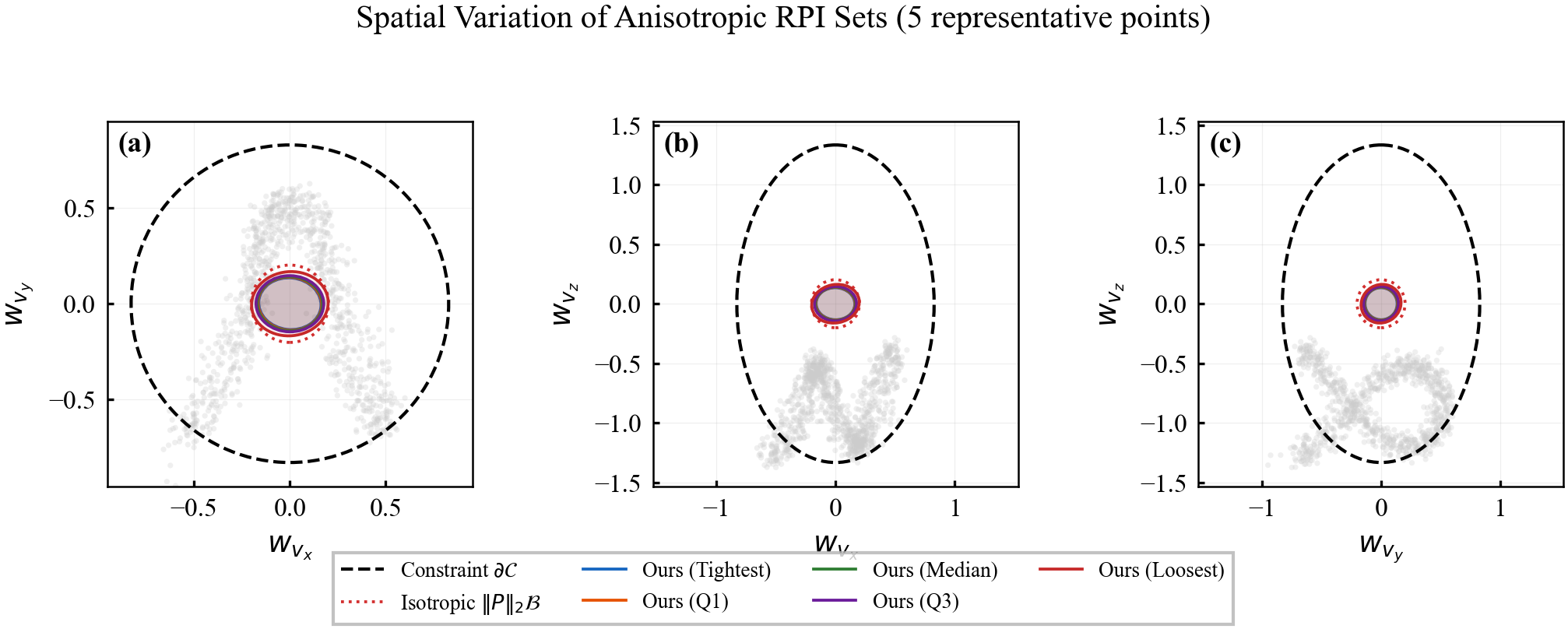
Remark 2 (Uniform vs. Arc-Wise Verification)
The uniform condition $(\gamma_{\mathrm{cl}}+1/r)\kappa_P\le 1$ is restrictive: since $\kappa_P := p_{\max}/p_{\min} \geq 1$ by definition, it requires $\gamma_{\mathrm{cl}} + 1/r \leq 1$, i.e., $r \geq 1/(1-\gamma_{\mathrm{cl}})$, which is exactly the template inflation factor. Thus the uniform condition is satisfiable with $\kappa_P = 1$ (isotropic fields) but becomes restrictive for highly anisotropic fields with $\kappa_P \gg 1$. The operative verification is the arc-wise criterion of Theorem 3, which exploits local ratios $p_i^+/p_j^-$ between neighboring regions. On a sufficiently fine grid, these local ratios approach unity even when the global condition number is large.
Graph-Based Discretization for Finite Verification
Assumption 4 (Graph Completeness)
The graph $\mathcal{G}=(\mathcal{V},\mathcal{A})$ captures all dynamically feasible transitions: for any closed-loop trajectory, if $(\mathbf{x}_k,\mathbf{u}_k)\in\mathcal{R}_i$ and $(\mathbf{x}_{k+1},\mathbf{u}_{k+1})\in\mathcal{R}_j$, then $(i,j)\in\mathcal{A}$.
Remark (Constructive graph construction)
In the implementation, $\mathcal{V}$ is constructed by clustering the sampled operating points using $k$-means, and arcs are initialized from consecutive closed-loop transitions in the rollout data. To make Assumption 4 constructive rather than empirical, each observed arc is enlarged by an interval over-approximation of the reachable successor set using the spectral bounds below; this may add spurious arcs, but spurious arcs only strengthen the verification problem because every added arc must also satisfy the invariance test. For the quadrotor benchmark: $k$-means with $N_v = 30$ yields $|\mathcal{A}| = 63$ arcs.
Definition 6 (Region Diameter and Lipschitz Deviation)
For each region $\mathcal{R}_i$: (1) diameter: $\mathrm{diam}(\mathcal{R}_i):=\sup_{\mathbf{z},\mathbf{z}'\in\mathcal{R}_i}\|\mathbf{z}-\mathbf{z}'\|_2$; (2) Lipschitz deviation bound: $\delta_i:=L_P\cdot\mathrm{diam}(\mathcal{R}_i)$.
Lemma 6 (Eigenvalue Bounds within Regions)
For any $\mathbf{z}\in\mathcal{R}_i$: $\lambda_{\max}(\mathbf{P}(\mathbf{z}))\le\lambda_{\max}(\mathbf{P}_i)+\delta_i$ and $\lambda_{\min}(\mathbf{P}(\mathbf{z}))\ge\lambda_{\min}(\mathbf{P}_i)-\delta_i$.
Goal. Bound $\lambda_{\max}(\mathbf{P}(\mathbf{z}))$ from above and $\lambda_{\min}(\mathbf{P}(\mathbf{z}))$ from below for all $\mathbf{z} \in \mathcal{R}_i$.
Step 1 (Lipschitz bound on matrix perturbation). By Assumption 2, the field $\mathbf{P}$ is Lipschitz with constant $L_P$. For any $\mathbf{z} \in \mathcal{R}_i$, the node $\mathbf{z}_i$ satisfies $\|\mathbf{z} - \mathbf{z}_i\|_2 \le \mathrm{rad}(\mathcal{R}_i)$, so:
Step 2 (Write as symmetric perturbation). Define the perturbation $\mathbf{E} := \mathbf{P}(\mathbf{z}) - \mathbf{P}_i$. Since both $\mathbf{P}(\mathbf{z})$ and $\mathbf{P}_i$ are symmetric (they are in $\mathbb{S}^n_{++}$), $\mathbf{E} \in \mathbb{S}^n$ with $\|\mathbf{E}\|_2 \le \delta_i$. We can write $\mathbf{P}(\mathbf{z}) = \mathbf{P}_i + \mathbf{E}$.
Step 3 (Apply Weyl's inequality for $\lambda_{\max}$). Weyl's eigenvalue perturbation inequality states: for symmetric $\mathbf{A}, \mathbf{B} \in \mathbb{S}^n$,
Here $\lambda_i$ denotes the $i$-th eigenvalue (ordered). In particular, both the maximum and minimum eigenvalues can shift by at most $\|\mathbf{B}\|_2$.
Why it matters. We know $\mathbf{P}(\mathbf{z})$ exactly only at grid nodes. Within each region, Weyl's inequality (combined with Lipschitz continuity) ensures eigenvalues stay within known bounds, enabling finite verification of invariance over the entire continuous domain.
Definition 7 (Spectral Bound Parameters)
For each node $i\in\mathcal{V}$: $p_i^+:=\lambda_{\max}(\mathbf{P}_i)+\delta_i$ (upper bound on $\|\mathbf{P}(\mathbf{z})\|_2$ for $\mathbf{z}\in\mathcal{R}_i$) and $p_i^-:=\lambda_{\min}(\mathbf{P}_i)-\delta_i$ (lower bound on $\lambda_{\min}(\mathbf{P}(\mathbf{z}))$ for $\mathbf{z}\in\mathcal{R}_i$).
Assumption 5 (Grid Fineness)
The partition $\{\mathcal{R}_i\}$ is sufficiently fine such that $\delta_i<\lambda_{\min}(\mathbf{P}_i)$ for all $i\in\mathcal{V}$, ensuring $p_i^->0$.
Lemma 7 (Spectral Norm Bounds for Matrix Products)
For any $\mathbf{z}\in\mathcal{R}_i$ and $\mathbf{z}'\in\mathcal{R}_j$: $\|\mathbf{M}\|_2\le\frac{p_i^+}{p_j^-}\gamma_{\mathrm{cl}}$ and $\|\mathbf{N}\|_2\le\frac{1}{r}\frac{p_i^+}{p_j^-}$.
Goal. Bound $\|\mathbf{M}\|_2$ and $\|\mathbf{N}\|_2$ using only node-computable quantities $p_i^+, p_j^-$.
Step 1 (Upper bound on $\|\mathbf{P}(\mathbf{z})\|_2$). For $\mathbf{z} \in \mathcal{R}_i$, since $\mathbf{P}(\mathbf{z}) \in \mathbb{S}^n_{++}$, its spectral norm equals its largest eigenvalue:
Step 2 (Upper bound on $\|\mathbf{P}(\mathbf{z}')^{-1}\|_2$). For $\mathbf{z}' \in \mathcal{R}_j$, Lemma 6 gives $\lambda_{\min}(\mathbf{P}(\mathbf{z}')) \ge p_j^-$. For a positive definite matrix, the spectral norm of its inverse is the reciprocal of its smallest eigenvalue:
This is well-defined since $p_j^- > 0$ by Assumption 5.
Step 3 (Bound $\|\mathbf{M}\|_2$ via submultiplicativity). Recall $\mathbf{M} = \mathbf{P}(\mathbf{z}')^{-1}\mathbf{A}_{\mathrm{cl}}\mathbf{P}(\mathbf{z})$. The spectral norm is submultiplicative ($\|\mathbf{A}\mathbf{B}\|_2 \le \|\mathbf{A}\|_2 \|\mathbf{B}\|_2$), so:
Step 5 (Conclude). Both bounds depend only on the spectral bound parameters $p_i^+$ and $p_j^-$ (and the template inflation factor $r$), which are computable from the node values $\lambda_{\max}(\mathbf{P}_i), \lambda_{\min}(\mathbf{P}_j)$ and the Lipschitz radii $\delta_i, \delta_j$. No evaluation of $\mathbf{P}(\cdot)$ at interior points of $\mathcal{R}_i$ or $\mathcal{R}_j$ is needed. $\square$
Main Discretization Theorem
Theorem 3 (Discrete Graph Invariance via Spectral Bounds)
Let $\mathcal{G}=(\mathcal{V},\mathcal{A})$ satisfy Assumptions 4-5. If for every arc $(i,j)\in\mathcal{A}$:
then the tube field $\boldsymbol{\Omega}(\mathbf{x},\mathbf{u})=\mathbf{P}(\mathbf{x},\mathbf{u})\bar{\boldsymbol{\Omega}}$ with $\bar{\boldsymbol{\Omega}}=r\mathcal{B}_2^n$ is locally RPI over $\mathcal{Z}$.
Goal. Show that the spectral edge condition implies the invariance condition from Theorem 1 for all continuous transitions, reducing infinite verification to a finite graph check.
Step 1 (Reduce to the norm condition). With templates $\bar{\boldsymbol{\Omega}} = r\mathcal{B}_2^n$ and $\bar{\mathbf{W}} = \mathcal{B}_2^n$, by Theorem 2 it suffices to show that for every transition $\mathbf{z} = (\mathbf{x},\mathbf{u}) \in \mathcal{R}_i \to \mathbf{z}' = (\mathbf{x}',\mathbf{u}') \in \mathcal{R}_j$ with $(i,j) \in \mathcal{A}$:
where $\mathbf{M} := \mathbf{P}(\mathbf{z}')^{-1}\mathbf{A}_{\mathrm{cl}}\mathbf{P}(\mathbf{z})$ and $\mathbf{N} := \tfrac{1}{r}\mathbf{P}(\mathbf{z}')^{-1}\mathbf{P}(\mathbf{z})$.
Step 2 (Apply triangle inequality). For any $\boldsymbol{\xi}', \boldsymbol{\eta}$ with $\|\boldsymbol{\xi}'\|_2 \le 1$ and $\|\boldsymbol{\eta}\|_2 \le 1$:
This holds for all $\boldsymbol{\xi}', \boldsymbol{\eta} \in \mathcal{B}_2^n$ and for all continuous $\mathbf{z} \in \mathcal{R}_i$, $\mathbf{z}' \in \mathcal{R}_j$ (not just at the nodes).
Step 6 (Completeness of the graph). Assumption 4 guarantees that for every feasible transition $(\mathbf{x},\mathbf{u}) \to (\mathbf{x}',\mathbf{u}')$, there exists an arc $(i,j) \in \mathcal{A}$ covering it. Therefore the norm condition is satisfied for all transitions in $\mathcal{Z}$, not just those between specific nodes.
Conclusion. By Theorem 1, satisfaction of the norm condition for all transitions implies local RPI of $\boldsymbol{\Omega}(\mathbf{z}) = \mathbf{P}(\mathbf{z})r\mathcal{B}_2^n$. The infinite verification over a continuous domain has been reduced to checking the scalar inequality $\frac{p_i^+}{p_j^-}(\gamma_{\mathrm{cl}} + 1/r) \le 1$ at each of the finitely many arcs $(i,j) \in \mathcal{A}$. $\square$
Remark 3 (Comparison with the Full LMI Condition)
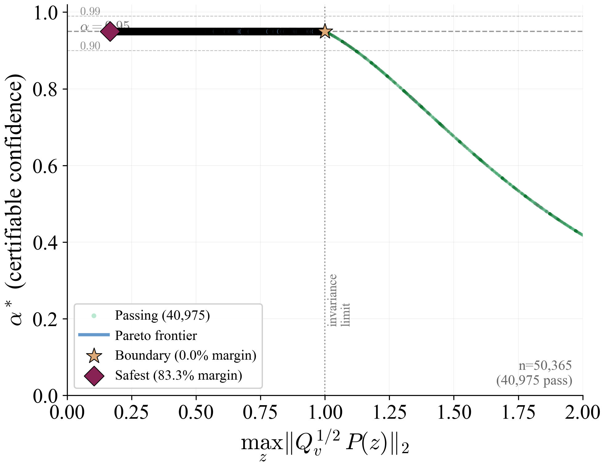
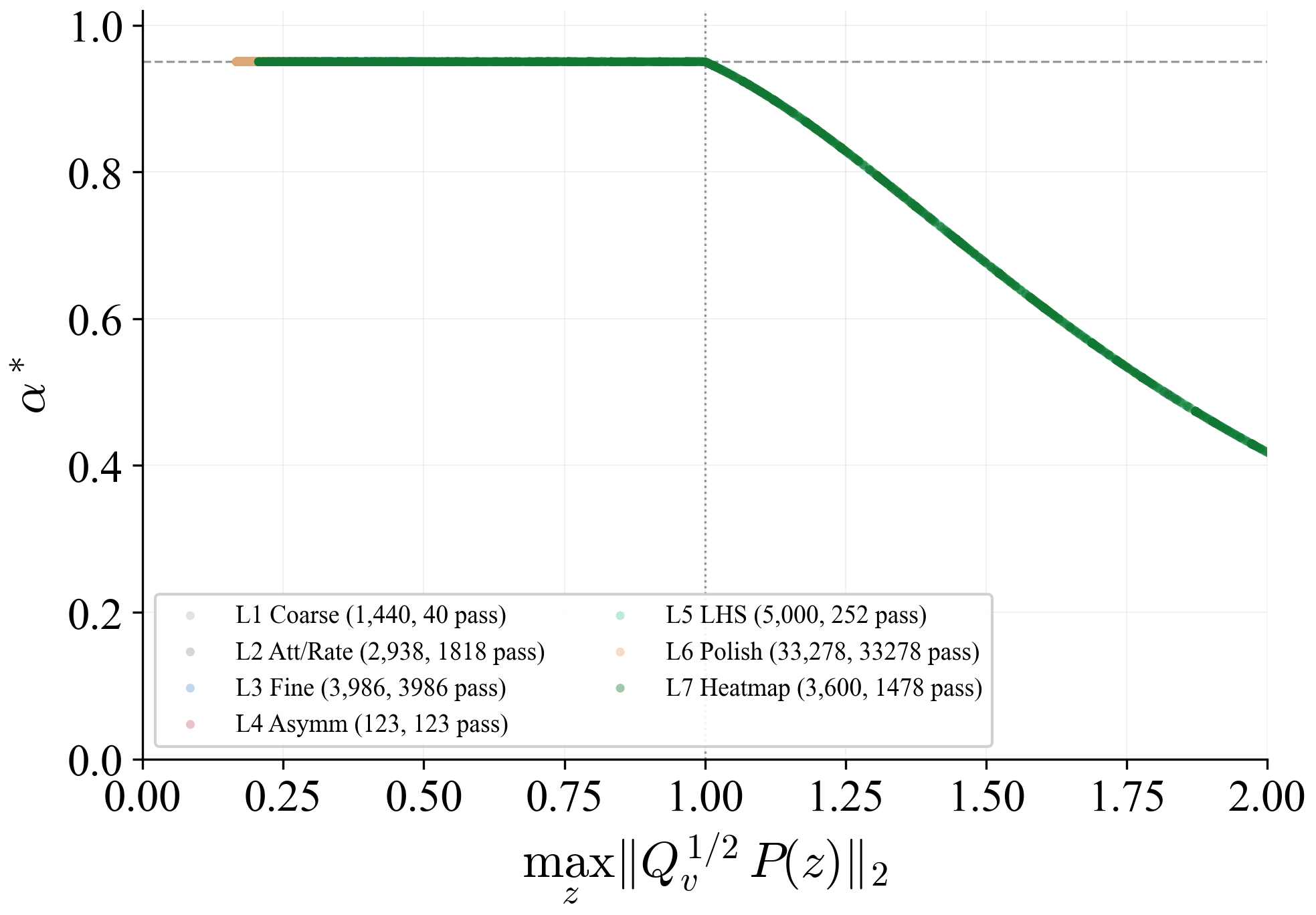
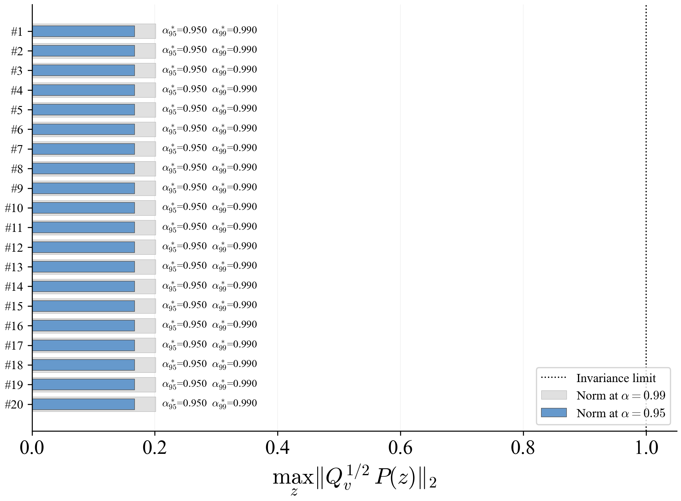
The arc-wise spectral condition is a conservative upper-bound version of the full LMI in Theorem 2. It replaces the exact matrices $\mathbf{M}$ and $\mathbf{N}$ by norm bounds and then applies the triangle inequality. This loses directional information in the Minkowski sum, but gives a scalar certificate that is easy to check on graph arcs. In the quadrotor benchmark, the per-point weighted norms lie in $[0.279,\,0.639]$, so the verified instances remain well below the unit threshold despite the conservative bound.
Remark (Scalability)
Verification is offline and scales with the feature dimension of $\mathbf{P}(\cdot)$, not the full state-input space. For the 12-state quadrotor, disturbances enter only the 3D velocity subspace, so the effective partition dimension is $3 + 4 = 7$ (velocity + control features), not $12 + 4 = 16$. A full dense grid in this subspace is subject to the curse of dimensionality, motivating disturbance-active subspaces, adaptive clustering, or sparse graph refinement. The quadrotor uses a 30-node, 63-arc graph in the three velocity components. Online, the graph is not traversed: evaluation is one cached GP covariance query and one $n_w \times n_w$ square root, about 0.1 ms for $N_{\mathrm{gp}} \le 300$, $n_w = 3$.
is feasible for some $\lambda_1,\lambda_2 \geq 0$ with $\lambda_1+\lambda_2\leq 1$, then the tube field is locally RPI.
Goal. Show that the scalar-bound LMI implies the full LMI of Theorem 2 for all $\mathbf{M},\mathbf{N}$ satisfying the spectral bounds.
From Lemma 7, $\|\mathbf{M}\|_2 \leq \bar{M}_{ij}$ and $\|\mathbf{N}\|_2 \leq \bar{N}_{ij}$. Therefore, for any vectors $\boldsymbol{\xi},\boldsymbol{\eta}$,
for all $\boldsymbol{\xi},\boldsymbol{\eta}$, with $\lambda_1,\lambda_2\ge0$ and $\lambda_1+\lambda_2\le1$. Hence the full Theorem 2 LMI holds for all matrices satisfying the norm bounds.
For scalars, feasibility of this LMI with $\lambda_1,\lambda_2\ge0$ and $\lambda_1+\lambda_2\le1$ is equivalent to $\bar{M}_{ij}+\bar{N}_{ij}\le1$. Thus the scalar-bound LMI recovers the same arc-wise spectral condition. The full LMI can still be less conservative when evaluated with the actual matrices $\mathbf{M}$ and $\mathbf{N}$ rather than only their scalar norm bounds. $\square$
Existence of Admissible Parameter Fields
We establish that the set of admissible parameter fields is non-empty and carries a partial order under the Löwner ordering, with smaller fields yielding tighter tubes. Define the admissible set
$$\mathscr{A} := \bigl\{\mathbf{P}: \mathcal{Z} \to \mathbb{S}^n_{++} \;\big|\; \text{the spectral condition holds for all } (i,j) \in \mathcal{A}\bigr\}.$$
Theorem (Existence via Isotropic Fallback)
Let $\gamma_{\mathrm{cl}} < 1$ and let $r = 1/(1 - \gamma_{\mathrm{cl}})$. Then for any $p > 0$, the constant isotropic field $\mathbf{P}(\mathbf{z}) \equiv p\,\mathbf{I}_n$ is admissible: $p\,\mathbf{I}_n \in \mathscr{A}$.
Step 1. For a constant field, $\delta_i = 0$ for all $i$, so $p_i^+ = p_i^- = p$ and $p_i^+/p_j^- = 1$ for all $(i,j) \in \mathcal{A}$.
Step 3. Since this holds for every arc, $p\,\mathbf{I}_n \in \mathscr{A}$. $\square$
Remark (Role of the Template Inflation Factor)
The equality $\gamma_{\mathrm{cl}} + 1/r = 1$ is not coincidental: the template inflation factor $r = 1/(1-\gamma_{\mathrm{cl}})$ is the minimal inflation ensuring $r\mathcal{B}_2^n$ is RPI for $(\mathbf{A}_{\mathrm{cl}}, \mathcal{B}_2^n)$, and the isotropic fallback saturates this bound with equality. Any non-constant field must therefore satisfy $p_i^+/p_j^- \leq 1/(\gamma_{\mathrm{cl}} + 1/r) = 1$, extracting invariance margin from the local regularity of $\mathbf{P}(\cdot)$ (i.e., from $\delta_i \to 0$ on fine grids) rather than from the template headroom. In particular, the Existence Theorem guarantees $\mathscr{A} \neq \emptyset$ but the isotropic field captures no directional structure; the GP-derived field must be certified separately via the arc-wise spectral condition.
Corollary (Admissibility of GP-Derived Field)
If the GP-induced field $\mathbf{P}^{\mathrm{GP}}(\mathbf{z})=c_{n,\alpha}\hat{\boldsymbol{\Sigma}}_w(\mathbf{z})^{1/2}$ satisfies Assumption 2 and the arc-wise spectral condition holds for all $(i,j)\in\mathcal{A}$, then $\mathbf{P}^{\mathrm{GP}} \in \mathscr{A}$.
Partial Order Structure
The Löwner order generalizes "less than or equal to" from scalars to symmetric matrices. For $\mathbf{A},\mathbf{B}\in\mathbb{S}^n$:
Why ordinary comparison fails. Consider $\mathbf{A}=\mathrm{diag}(5,1)$ and $\mathbf{B}=\mathrm{diag}(2,3)$. Entry-wise: $5>2$ but $1<3$. There is no consistent scalar ranking. The Löwner order resolves this by requiring the difference to be positive semidefinite in all directions simultaneously.
Partial order. Unlike scalars (which are totally ordered), matrices under $\preceq$ form only a partial order: some pairs are incomparable. But for the GP posterior covariance, data accumulation pushes the ordering consistently: $\hat{\boldsymbol{\Sigma}}_w^{(q+1)}\preceq\hat{\boldsymbol{\Sigma}}_w^{(q)}$ is guaranteed for all points.
Geometric meaning. For covariance matrices $\boldsymbol{\Sigma}_1\preceq\boldsymbol{\Sigma}_2$ (both positive definite), the ellipsoid $\boldsymbol{\Sigma}_1^{1/2}\mathcal{B}_2^n$ is contained inside $\boldsymbol{\Sigma}_2^{1/2}\mathcal{B}_2^n$ (see Proposition 2 for the proof). In our context: when the GP posterior covariance shrinks in the Löwner sense, the local tube ellipsoid shrinks with it.
Caution. For generic SPD matrices, $\mathbf{P}_1\preceq\mathbf{P}_2$ does not in general imply $\mathbf{P}_1\mathcal{B}_2^n\subseteq\mathbf{P}_2\mathcal{B}_2^n$. The containment requires the additional structure $\mathbf{P}_i=c\,\boldsymbol{\Sigma}_i^{1/2}$ with $\boldsymbol{\Sigma}_1\preceq\boldsymbol{\Sigma}_2$; see the warning box after Proposition 2.
Proposition 2 (Ordering of Admissible Fields)
Let $\boldsymbol{\Sigma}_1,\boldsymbol{\Sigma}_2:\mathcal{Z}\to\mathbb{S}^n_{++}$ with $\boldsymbol{\Sigma}_1(\mathbf{z})\preceq\boldsymbol{\Sigma}_2(\mathbf{z})$ pointwise, and let $\mathbf{P}_i := c\,\boldsymbol{\Sigma}_i^{1/2}$ for a scalar $c > 0$. If both $\mathbf{P}_1,\mathbf{P}_2$ satisfy the spectral invariance condition, then: (1) $\boldsymbol{\Omega}_1(\mathbf{z})\subseteq\boldsymbol{\Omega}_2(\mathbf{z})$ for all $\mathbf{z}$; (2) both are locally RPI but $\boldsymbol{\Omega}_1$ gives tighter tubes.
Why the hypothesis is on $\boldsymbol{\Sigma}_1 \preceq \boldsymbol{\Sigma}_2$ rather than $\mathbf{P}_1 \preceq \mathbf{P}_2$.
For general SPD matrices, the Löwner ordering $\mathbf{P}_1 \preceq \mathbf{P}_2$ does not imply $\mathbf{P}_1\mathcal{B}_2^n \subseteq \mathbf{P}_2\mathcal{B}_2^n$. The matrix $\mathbf{P}_2^{-1}\mathbf{P}_1$ is generically non-symmetric, so its eigenvalues being $\le 1$ does not bound its spectral norm (largest singular value). The hypothesis $\boldsymbol{\Sigma}_1 \preceq \boldsymbol{\Sigma}_2$ with $\mathbf{P}_i = c\,\boldsymbol{\Sigma}_i^{1/2}$ provides the additional algebraic structure needed: the key matrix $\boldsymbol{\Sigma}_2^{-1/2}\boldsymbol{\Sigma}_1^{1/2}$ has singular values bounded by 1 because its $\mathbf{C}\mathbf{C}^\top$ form is SPD and $\preceq \mathbf{I}$. This is exactly the structure present in the paper, where $\mathbf{P} = c_{n,\alpha}\hat{\boldsymbol{\Sigma}}_w^{1/2}$ and the GP variance reduction gives $\hat{\boldsymbol{\Sigma}}_w^{(q+1)} \preceq \hat{\boldsymbol{\Sigma}}_w^{(q)}$ directly.
Goal. Show that if $\boldsymbol{\Sigma}_1(\mathbf{z}) \preceq \boldsymbol{\Sigma}_2(\mathbf{z})$ pointwise and $\mathbf{P}_i = c\,\boldsymbol{\Sigma}_i^{1/2}$, then (1) $\boldsymbol{\Omega}_1 := \mathbf{P}_1\bar{\boldsymbol{\Omega}} \subseteq \mathbf{P}_2\bar{\boldsymbol{\Omega}} =: \boldsymbol{\Omega}_2$ pointwise, and (2) both are locally RPI.
Part 1: Set containment $\boldsymbol{\Sigma}_1^{1/2}\mathcal{B}_2^n \subseteq \boldsymbol{\Sigma}_2^{1/2}\mathcal{B}_2^n$.
Since $\mathbf{P}_i = c\,\boldsymbol{\Sigma}_i^{1/2}$ and the template $\bar{\boldsymbol{\Omega}} = r\mathcal{B}_2^n$, we have $\boldsymbol{\Omega}_i = cr\,\boldsymbol{\Sigma}_i^{1/2}\mathcal{B}_2^n$. The positive scalars $c,r$ factor out identically on both sides, so it suffices to prove $\boldsymbol{\Sigma}_1^{1/2}\mathcal{B}_2^n \subseteq \boldsymbol{\Sigma}_2^{1/2}\mathcal{B}_2^n$.
Step 1a (Pick arbitrary element). Let $\mathbf{e} \in \boldsymbol{\Sigma}_1^{1/2}\mathcal{B}_2^n$. Then there exists $\boldsymbol{\xi} \in \mathcal{B}_2^n$ ($\|\boldsymbol{\xi}\|_2 \le 1$) such that $\mathbf{e} = \boldsymbol{\Sigma}_1^{1/2}\boldsymbol{\xi}$.
Step 1b (Express in $\boldsymbol{\Sigma}_2^{1/2}$-coordinates). Define $\boldsymbol{\zeta} := \boldsymbol{\Sigma}_2^{-1/2}\mathbf{e} = \boldsymbol{\Sigma}_2^{-1/2}\boldsymbol{\Sigma}_1^{1/2}\boldsymbol{\xi}$. We need to show $\|\boldsymbol{\zeta}\|_2 \le 1$, which would mean $\mathbf{e} = \boldsymbol{\Sigma}_2^{1/2}\boldsymbol{\zeta} \in \boldsymbol{\Sigma}_2^{1/2}\mathcal{B}_2^n$.
Step 1c (Form $\mathbf{C}\mathbf{C}^\top$ from the covariance ordering). Define $\mathbf{C} := \boldsymbol{\Sigma}_2^{-1/2}\boldsymbol{\Sigma}_1^{1/2}$. Because $\boldsymbol{\Sigma}_1^{1/2}$ is symmetric (it is the unique SPD square root), we can compute:
This is a congruence of $\boldsymbol{\Sigma}_1$ by the invertible matrix $\boldsymbol{\Sigma}_2^{-1/2}$. Congruences preserve the Löwner ordering: from $\boldsymbol{\Sigma}_1 \preceq \boldsymbol{\Sigma}_2$,
Step 1d (Bound the spectral norm of $\mathbf{C}$). The matrix $\mathbf{C}\mathbf{C}^\top$ is symmetric positive semidefinite with all eigenvalues $\le 1$. The squared spectral norm of $\mathbf{C}$ equals the largest eigenvalue of $\mathbf{C}\mathbf{C}^\top$:
This step is correct precisely because $\mathbf{C}\mathbf{C}^\top$ is symmetric — for a symmetric matrix, the spectral norm equals the spectral radius. (For a generic non-symmetric matrix, eigenvalues $\le 1$ would not imply $\|\cdot\|_2 \le 1$.)
Therefore $\boldsymbol{\zeta} \in \mathcal{B}_2^n$ and $\mathbf{e} = \boldsymbol{\Sigma}_2^{1/2}\boldsymbol{\zeta} \in \boldsymbol{\Sigma}_2^{1/2}\mathcal{B}_2^n$. Scaling by $cr$ gives $\mathbf{P}_1\bar{\boldsymbol{\Omega}} \subseteq \mathbf{P}_2\bar{\boldsymbol{\Omega}}$.
Part 2: Both fields are RPI. Both $\mathbf{P}_1$ and $\mathbf{P}_2$ satisfy the spectral invariance condition by assumption. Theorem 3 then directly implies both $\boldsymbol{\Omega}_1$ and $\boldsymbol{\Omega}_2$ are locally RPI. The containment from Part 1 means $\boldsymbol{\Omega}_1$ provides strictly tighter uncertainty tubes. $\square$
Monotone Tube Contraction
A function $f:\mathbb{R}_+\to\mathbb{R}_+$ is operator monotone if, whenever $\mathbf{A}\preceq\mathbf{B}$ (in the Löwner order), we also have $f(\mathbf{A})\preceq f(\mathbf{B})$. Here $f(\mathbf{A})$ is defined via the spectral theorem: if $\mathbf{A}=\mathbf{V}\boldsymbol{\Lambda}\mathbf{V}^\top$, then $f(\mathbf{A})=\mathbf{V}f(\boldsymbol{\Lambda})\mathbf{V}^\top$.
Key fact (Löwner-Heinz theorem): The map $t\mapsto t^r$ is operator monotone for $r\in[0,1]$. In particular, the square root ($r=1/2$) is operator monotone: $\mathbf{A}\preceq\mathbf{B}\Rightarrow\mathbf{A}^{1/2}\preceq\mathbf{B}^{1/2}$.
Caution: For $r>1$, operator monotonicity fails. For example, $\mathbf{A}\preceq\mathbf{B}$ does NOT imply $\mathbf{A}^2\preceq\mathbf{B}^2$ in general. This is why the square root step is essential and non-trivial.
Role in this paper. From $\hat{\boldsymbol{\Sigma}}_w^{(q+1)}\preceq\hat{\boldsymbol{\Sigma}}_w^{(q)}$ (posterior variance reduces with data), operator monotonicity gives $[\hat{\boldsymbol{\Sigma}}_w^{(q+1)}]^{1/2}\preceq[\hat{\boldsymbol{\Sigma}}_w^{(q)}]^{1/2}$, and hence $\mathbf{P}^{(q+1)}\preceq\mathbf{P}^{(q)}$, which yields tube contraction.
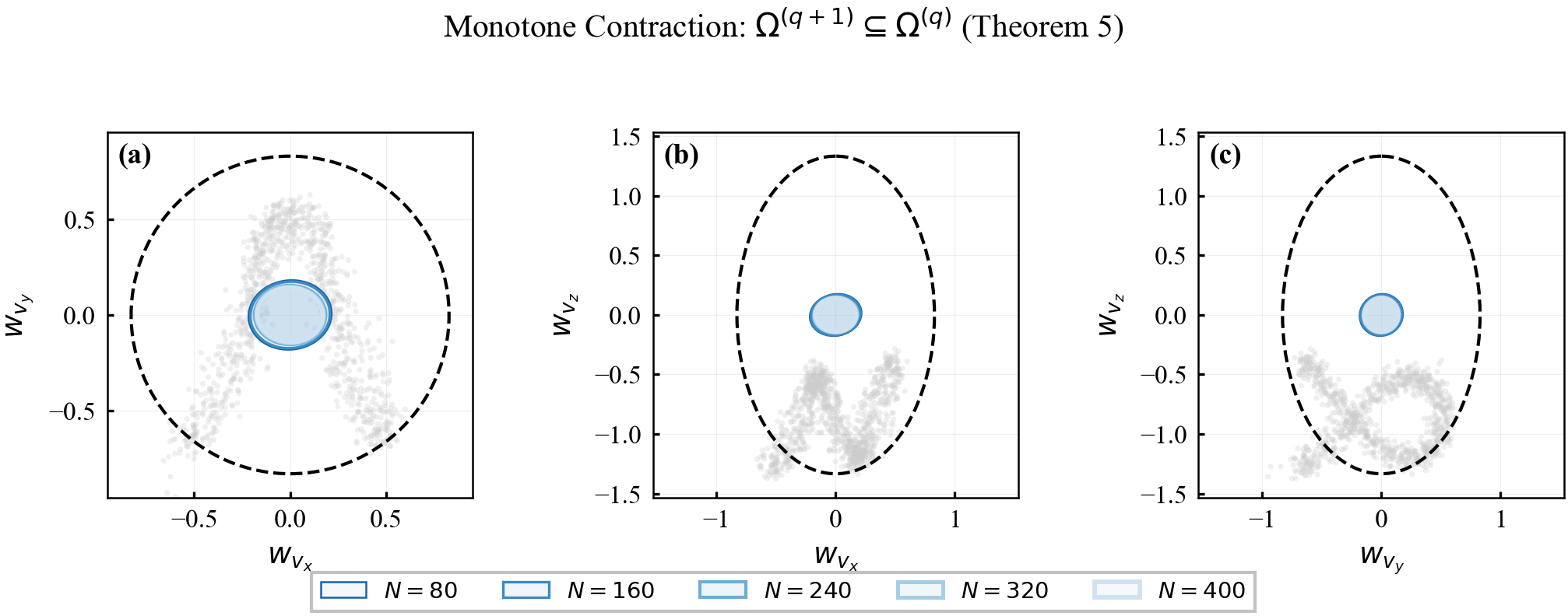
Theorem 5 (Monotone Tube Contraction under Data Accumulation)
As data accumulate across learning epochs $q=0,1,2,\ldots$:
$\hat{\boldsymbol{\Sigma}}_w^{(q+1)}(\mathbf{z})\preceq\hat{\boldsymbol{\Sigma}}_w^{(q)}(\mathbf{z})$ for all $\mathbf{z}\in\mathcal{Z}$ (variance reduction).
$\mathbf{P}^{(q+1)}(\mathbf{z})\preceq\mathbf{P}^{(q)}(\mathbf{z})$ for all $\mathbf{z}\in\mathcal{Z}$ (anisotropy field shrinkage).
$\boldsymbol{\Omega}^{(q+1)}(\mathbf{z})\subseteq\boldsymbol{\Omega}^{(q)}(\mathbf{z})$ for all $\mathbf{z}\in\mathcal{Z}$ (tube contraction).
Part 2: Anisotropy field shrinkage $\mathbf{P}^{(q+1)} \preceq \mathbf{P}^{(q)}$.
Step 2a (Recall the definition). The anisotropy field is $\mathbf{P}^{(q)}(\mathbf{z}) := c_{n,\alpha}[\hat{\boldsymbol{\Sigma}}_w^{(q)}(\mathbf{z})]^{1/2}$, where $c_{n,\alpha} > 0$ is a scalar confidence scaling factor.
Step 2b (Invoke the Löwner-Heinz theorem). The matrix square root $t \mapsto t^{1/2}$ is operator monotone on $\mathbb{S}^n_+$ (Löwner-Heinz theorem with exponent $r = 1/2$). This means:
Step 2c (Apply to the posterior covariance). Part 1 established $\hat{\boldsymbol{\Sigma}}_w^{(q+1)}(\mathbf{z}) \preceq \hat{\boldsymbol{\Sigma}}_w^{(q)}(\mathbf{z})$. Applying operator monotonicity of the square root:
Step 2d (Scale by the confidence factor). Multiplying both sides by $c_{n,\alpha} > 0$ preserves the ordering (positive scalar multiplication is order-preserving):
Part 3: Tube contraction $\boldsymbol{\Omega}^{(q+1)} \subseteq \boldsymbol{\Omega}^{(q)}$.
Step 3a (Invoke Proposition 2). Part 1 established the covariance ordering $\hat{\boldsymbol{\Sigma}}_w^{(q+1)}(\mathbf{z}) \preceq \hat{\boldsymbol{\Sigma}}_w^{(q)}(\mathbf{z})$ for all $\mathbf{z} \in \mathcal{Z}$. Since $\mathbf{P}^{(q)} = c_{n,\alpha}[\hat{\boldsymbol{\Sigma}}_w^{(q)}]^{1/2}$, Proposition 2 (with $\boldsymbol{\Sigma}_i = \hat{\boldsymbol{\Sigma}}_w^{(i)}$ and $c = c_{n,\alpha}$) gives set containment:
Step 3b (Geometric interpretation). Each ellipsoidal cross-section $\boldsymbol{\Omega}^{(q+1)}(\mathbf{z})$ is nested inside $\boldsymbol{\Omega}^{(q)}(\mathbf{z})$, with the nesting preserving the anisotropic shape. The semi-axes of the ellipsoid shrink monotonically in every direction as data accumulate, with directions of high data density shrinking fastest. $\square$
Goal. Show $\hat{\boldsymbol{\Sigma}}_w^{(q+1)}(\mathbf{z}_*)\preceq\hat{\boldsymbol{\Sigma}}_w^{(q)}(\mathbf{z}_*)$ for all $\mathbf{z}_*\in\mathcal{Z}$ using Schur complement properties.
Step 1 (GP posterior as Schur complement). The GP posterior covariance at a test point $\mathbf{z}_*$ conditioned on data $\mathcal{D}^{(q)}$ is:
This is precisely the Schur complement of the $(\mathcal{D},\mathcal{D})$ block in the joint covariance matrix. Consider the joint distribution of $[\mathbf{w}(\mathbf{z}_*), \mathbf{y}_{\mathcal{D}^{(q)}}]$ where $\mathbf{y} = \mathbf{w} + \boldsymbol{\epsilon}$ ($\boldsymbol{\epsilon} \sim \mathcal{N}(\mathbf{0}, \sigma_n^2\mathbf{I})$). The joint covariance is:
Step 2 (Augment the conditioning set). At epoch $q{+}1$, one new data point is added: $\mathcal{D}^{(q+1)} = \mathcal{D}^{(q)} \cup \{(\mathbf{z}^{\mathrm{new}}, \mathbf{y}^{\mathrm{new}})\}$. The joint covariance becomes:
In words: the Schur complement of a larger principal submatrix is always $\preceq$ the Schur complement of a smaller one. This is because conditioning on more variables can only reduce (or maintain) the conditional variance.
Step 4 (Identify the blocks). In our setting: $\mathbf{A} = \boldsymbol{\Sigma}_{**}$ (test point block), $\mathbf{D} = \boldsymbol{\Sigma}_{\mathcal{D}\mathcal{D}} + \sigma_n^2\mathbf{I}$ (old data block), $\mathbf{F} = \boldsymbol{\Sigma}_{\mathrm{new,new}} + \sigma_n^2\mathbf{I}$ (new data block). Then:
$\mathbf{G}^{(q+1)} / \begin{bmatrix}\mathbf{D} & \mathbf{E} \\ \mathbf{E}^\top & \mathbf{F}\end{bmatrix} = \hat{\boldsymbol{\Sigma}}_w^{(q+1)}(\mathbf{z}_*)$ (posterior with all data),
$\mathbf{G}^{(q)} / \mathbf{D} = \hat{\boldsymbol{\Sigma}}_w^{(q)}(\mathbf{z}_*)$ (posterior with old data only).
Step 5 (Conclude). By the Schur complement monotonicity lemma:
This is the most conceptually clean proof: it uses only the fact that conditioning on more data (enlarging the Schur complement's denominator block) can only reduce uncertainty. $\square$
Goal. Show $\hat{\boldsymbol{\Sigma}}_w^{(q+1)}(\mathbf{z}_*)\preceq\hat{\boldsymbol{\Sigma}}_w^{(q)}(\mathbf{z}_*)$ for all $\mathbf{z}_*\in\mathcal{Z}$ using information (precision) matrices.
Step 1 (Define the information matrix). The information matrix (precision matrix) at $\mathbf{z}_*$ given data $\mathcal{D}^{(q)}$ is:
Higher information (larger $\boldsymbol{\Lambda}$ in the Löwner sense) corresponds to lower uncertainty (smaller $\hat{\boldsymbol{\Sigma}}_w$).
Step 2 (Information update formula). When a new observation $(\mathbf{z}^{\mathrm{new}}, \mathbf{y}^{\mathrm{new}})$ is incorporated, the information matrix updates as:
where $\mathbf{H} \in \mathbb{R}^{n \times n}$ is the "observation model" matrix relating the test point to the new observation (derived from the GP cross-covariance structure), and $\boldsymbol{\Gamma} \succ \mathbf{0}$ is the innovation covariance. This is the multi-output generalization of the scalar information filter update.
Step 3 (Show the update is PSD). The update term $\mathbf{H}^\top\boldsymbol{\Gamma}^{-1}\mathbf{H}$ is positive semidefinite. For any $\mathbf{v} \in \mathbb{R}^n$:
Proof of reversal: If $\mathbf{A} \succeq \mathbf{B} \succ \mathbf{0}$, then for any $\mathbf{v} \ne \mathbf{0}$, set $\mathbf{u} = \mathbf{B}^{-1/2}\mathbf{v}$. We have $\mathbf{u}^\top\mathbf{B}^{1/2}\mathbf{A}^{-1}\mathbf{B}^{1/2}\mathbf{u} \le \mathbf{u}^\top\mathbf{u}$ (since $\mathbf{A}^{-1} \preceq \mathbf{B}^{-1}$ is equivalent to $\mathbf{B}^{1/2}\mathbf{A}^{-1}\mathbf{B}^{1/2} \preceq \mathbf{I}$, which follows from $\mathbf{B}^{-1/2}\mathbf{A}\mathbf{B}^{-1/2} \succeq \mathbf{I}$).
Step 6 (Conclude). Applying order reversal to Step 4:
This route is perhaps the most intuitive: data add information ($\boldsymbol{\Lambda}$ grows), and inversion converts information growth into uncertainty reduction. $\square$
This is a self-contained, step-by-step derivation of posterior covariance monotonicity via explicit block matrix inversion. It uses no abbreviations and shows every intermediate step.
Setup and Notation
Consider a multi-output GP with $n$ outputs under the Linear Model of Coregionalization (LMC). At epoch $q$, the dataset is $\mathcal{D}^{(q)}=\{(\mathbf{z}^{(j)},\mathbf{w}^{(j)})\}_{j=1}^{N_q}$. The GP posterior covariance at a test point $\mathbf{z}_*\in\mathcal{Z}$ is
where $\boldsymbol{\Sigma}_{**}:=K_{\mathrm{LMC}}(\mathbf{z}_*,\mathbf{z}_*)\in\mathbb{R}^{n\times n}$ is the prior covariance, $\boldsymbol{\Sigma}_{*\mathcal{D}^{(q)}}\in\mathbb{R}^{n\times nN_q}$ is the cross-covariance, $\boldsymbol{\Sigma}_{\mathcal{D}^{(q)}\mathcal{D}^{(q)}}\in\mathbb{R}^{nN_q\times nN_q}$ is the training kernel matrix, and $\sigma_n^2>0$ is the observation noise.
At epoch $q{+}1$, one new data point $(\mathbf{z}^{\mathrm{new}},\mathbf{w}^{\mathrm{new}})$ is added: $\mathcal{D}^{(q+1)}=\mathcal{D}^{(q)}\cup\{(\mathbf{z}^{\mathrm{new}},\mathbf{w}^{\mathrm{new}})\}$.
Goal: Prove $\hat{\boldsymbol{\Sigma}}_w^{(q+1)}(\mathbf{z}_*)\preceq\hat{\boldsymbol{\Sigma}}_w^{(q)}(\mathbf{z}_*)$ for all $\mathbf{z}_*\in\mathcal{Z}$.
The goal $\hat{\boldsymbol{\Sigma}}_w^{(q+1)}\preceq\hat{\boldsymbol{\Sigma}}_w^{(q)}$ is equivalent to $\boldsymbol{\Phi}^{(q+1)}\succeq\boldsymbol{\Phi}^{(q)}$ (since $\boldsymbol{\Sigma}_{**}$ is the same at both epochs).
For a block matrix $\mathbf{M}=\begin{bmatrix}\mathbf{A}&\mathbf{B}\\\mathbf{B}^\top&\mathbf{D}\end{bmatrix}$ with $\mathbf{A}$ invertible, the Schur complement of $\mathbf{A}$ is $\mathbf{S}:=\mathbf{D}-\mathbf{B}^\top\mathbf{A}^{-1}\mathbf{B}$. If $\mathbf{S}$ is invertible:
Key property: If the full matrix $\mathbf{M}\succ\mathbf{0}$ and $\mathbf{A}\succ\mathbf{0}$, then $\mathbf{S}\succ\mathbf{0}$.
Claim: $\boldsymbol{\Delta}\succ\mathbf{0}$. Since $\mathbf{M}_2\succ\mathbf{0}$ and $\mathbf{M}_1\succ\mathbf{0}$, the Schur complement characterization of positive definiteness gives $\boldsymbol{\Delta}\succ\mathbf{0}$.
Interpretation: Expanding, $\boldsymbol{\Delta}=\hat{\boldsymbol{\Sigma}}_w^{(q)}(\mathbf{z}^{\mathrm{new}})+\sigma_n^2\mathbf{I}_n$ (the posterior covariance at the new point, plus noise).
Lemma. For any $\mathbf{R}\in\mathbb{R}^{n\times n}$ and $\boldsymbol{\Delta}\succ\mathbf{0}$, the product $\mathbf{R}\boldsymbol{\Delta}^{-1}\mathbf{R}^\top\succeq\mathbf{0}$.
Proof. Since $\boldsymbol{\Delta}\succ\mathbf{0}$, we have $\boldsymbol{\Delta}^{-1}\succ\mathbf{0}$. For any $\mathbf{v}\in\mathbb{R}^n$, let $\mathbf{w}:=\mathbf{R}^\top\mathbf{v}$. Then:
Since $\boldsymbol{\Phi}^{(q)}=\boldsymbol{\Sigma}_{**}-\hat{\boldsymbol{\Sigma}}_w^{(q)}$ with the same $\boldsymbol{\Sigma}_{**}$:
$$\hat{\boldsymbol{\Sigma}}_w^{(q+1)}(\mathbf{z}_*)\preceq\hat{\boldsymbol{\Sigma}}_w^{(q)}(\mathbf{z}_*)\quad\text{for all }\mathbf{z}_*\in\mathcal{Z}.$$
GP Interpretation
The residual $\mathbf{R}$ and Schur complement $\boldsymbol{\Delta}$ have natural GP interpretations:
$\mathbf{R}=\mathrm{Cov}^{(q)}(\mathbf{w}(\mathbf{z}_*),\mathbf{w}(\mathbf{z}^{\mathrm{new}}))$ - the posterior cross-covariance between the test point and the new point.
$\boldsymbol{\Delta}=\mathrm{Var}^{(q)}(\mathbf{w}(\mathbf{z}^{\mathrm{new}}))+\sigma_n^2\mathbf{I}_n$ - the posterior variance at the new point, plus noise.
The improvement at $\mathbf{z}_*$ is proportional to how correlated $\mathbf{z}_*$ is with the new point (the $\mathbf{R}$ factors) and inversely proportional to how uncertain the new point itself is (the $\boldsymbol{\Delta}^{-1}$ factor). High residual correlation and low residual uncertainty yield the largest improvement; a fully redundant point ($\mathbf{R}=\mathbf{0}$) contributes nothing.
Scalar Sanity Check
For $n=1$ (single output), all "matrices" become scalars: $\mathbf{R}\to r$, $\boldsymbol{\Delta}\to\delta>0$. The formula becomes $\Phi^{(q+1)}-\Phi^{(q)}=r^2/\delta\ge 0$, recovering the standard scalar GP posterior variance update. $\square$
Remark 5 (Invariance Re-verification)
The spectral condition is not automatically preserved under tube contraction. Since $\mathbf{P}^{(q+1)}\preceq\mathbf{P}^{(q)}$ implies both $\lambda_{\max}$ and $\lambda_{\min}$ decrease, the ratio $p_i^+/p_j^-$ may increase or decrease depending on relative rates. The condition must be re-verified at each learning epoch.
Proposition 3 (Sufficient Condition for Invariance Preservation)
If at epoch $q$ the uniform condition $\frac{p_{\max}^{(q)}}{p_{\min}^{(q)}}\cdot(\|\mathbf{A}_{\mathrm{cl}}\|_2+1/r)\le 1$ holds, then the arc-wise condition is satisfied for all $(i,j)\in\mathcal{A}$.
Goal. Show that the uniform condition $\frac{p_{\max}^{(q)}}{p_{\min}^{(q)}}(\|\mathbf{A}_{\mathrm{cl}}\|_2 + 1/r) \le 1$ implies the arc-wise condition for every $(i,j) \in \mathcal{A}$.
Step 1 (Recall definitions). The global spectral bounds are:
The local spectral bounds from Definition 7 are $p_i^+ = \lambda_{\max}(\mathbf{P}_i) + \delta_i$ and $p_j^- = \lambda_{\min}(\mathbf{P}_j) - \delta_j$.
Step 2 (Bound $p_i^+$ from above). For any node $i$, by Lemma 6, $\lambda_{\max}(\mathbf{P}(\mathbf{z})) \le p_i^+$ for all $\mathbf{z} \in \mathcal{R}_i$. Since $p_{\max}^{(q)}$ is the supremum over all $\mathbf{z} \in \mathcal{Z} = \bigcup_i \mathcal{R}_i$:
$$p_i^+ \le p_{\max}^{(q)} \quad \text{for all } i \in \mathcal{V}.$$
(In fact $p_i^+$ could be larger than $\max_{\mathbf{z} \in \mathcal{R}_i} \lambda_{\max}(\mathbf{P}(\mathbf{z}))$ due to the Lipschitz over-approximation, but it is always bounded by the global maximum.)
Step 3 (Bound $p_j^-$ from below). Similarly, $\lambda_{\min}(\mathbf{P}(\mathbf{z})) \ge p_j^-$ for all $\mathbf{z} \in \mathcal{R}_j$. Since $p_{\min}^{(q)}$ is the infimum:
$$p_j^- \ge p_{\min}^{(q)} \quad \text{for all } j \in \mathcal{V}.$$
Step 4 (Form the ratio bound). For any arc $(i,j) \in \mathcal{A}$:
The last inequality is the uniform condition assumed in the proposition.
Step 5 (Conclude). Since this holds for every $(i,j) \in \mathcal{A}$, the arc-wise spectral condition of Theorem 3 is satisfied. Note that the uniform condition is sufficient but not necessary: individual arcs may satisfy $\frac{p_i^+}{p_j^-}(\|\mathbf{A}_{\mathrm{cl}}\|_2 + 1/r) \le 1$ even when the global ratio $p_{\max}^{(q)}/p_{\min}^{(q)}$ violates the uniform bound. $\square$
Remark 6 (Practical Persistence of Invariance)
Although the arc-wise condition requires re-verification, the uniform condition often persists in practice. The noise floor $\sigma_n^2$ prevents the denominator from vanishing, and as data accumulate in high-uncertainty regions, $p_{\max}^{(q)}$ typically decreases faster than $p_{\min}^{(q)}$, improving the condition number.
Two-Time-Scale Architecture
The verification condition requires the successor $(\mathbf{x}',\mathbf{u}')$ to evaluate $\mathbf{P}'$, yet $\mathbf{x}'$ depends on $\mathbf{w}\in\mathbb{W}(\mathbf{x},\mathbf{u})$, a circular dependency. We resolve this by freezing the GP-derived field $\mathbf{P}^{(q)}(\cdot)$ during each learning epoch $q$:
Train the GP to obtain $\hat{\boldsymbol{\Sigma}}_w^{(q)}$ and construct $\mathbf{P}^{(q)}=c_{n,\alpha}[\hat{\boldsymbol{\Sigma}}_w^{(q)}]^{1/2}$.
With $\mathbf{P}^{(q)}$ fixed, verify invariance via the graph-based spectral condition of Theorem 3.
Collect new data during operation.
Increment $q$ and repeat.
Unlike the lifted fixed-point method, which recomputes set geometry through iterative polytope operations, the proposed method updates only the anisotropy matrix field. Online tube evaluation reduces to one GP covariance query and one small matrix square root per operating point ($O(N_{\mathrm{gp}}^2)$ with cached Cholesky factors, where $N_{\mathrm{gp}}$ is the capped training subset size), independent of the MPC horizon, graph size, and learning epoch count.
Computational Complexity Analysis
We now provide a detailed phase-by-phase complexity breakdown. Let $n_x$, $n_u$, $n_w$ denote the state, input, and disturbance dimensions respectively, $N_{\mathrm{gp}}$ the (capped) GP training set size, $R$ the number of latent GPs in the LMC kernel, $|\mathcal{V}|$ the number of graph vertices, and $|\mathcal{A}|$ the number of graph arcs. For the quadrotor system: $n_x{=}12$, $n_u{=}4$, $n_w{=}3$, $R{=}3$, $N_{\mathrm{gp}}{\le}300$, $|\mathcal{V}|{=}30$, $|\mathcal{A}|{=}63$.
I. Offline Phase (One-Time or Per-Epoch)
The offline phase runs once at initialization (Steps 1–2) and is repeated each learning epoch (Steps 3–4).
Step
Operation
Cost
Notes
1. Template pair
Solve DARE for $\mathbf{S}_\infty$; compute $\bar{\mathbf{T}},\bar{\mathbf{T}}_w$ via~\eqref{eq:template_inflation}
$O(n_x^3)$
One-time; standard Schur decomposition. For $n_x{=}12$: negligible (${\lt}1\,$ms).
LMC kernel hyperparameter optimization via marginal likelihood
$O(E_{\mathrm{gp}}\,N_{\mathrm{gp}}^3\,R\,n_w)$
$E_{\mathrm{gp}}{=}500$ L-BFGS epochs. Dominated by Cholesky factorization of the $N_{\mathrm{gp}}\times N_{\mathrm{gp}}$ kernel matrix. With $N_{\mathrm{gp}}{\le}300$: typically ${\sim}30\,$s on GPU (GPyTorch).
4. Graph construction
$k$-means clustering of training data into $|\mathcal{V}|$ clusters; arcs from consecutive trajectory transitions
$O(N_{\mathrm{gp}}\,|\mathcal{V}|\,d)$
$d{=}n_x{+}n_u{=}16$ feature dimensions. For $N_{\mathrm{gp}}{=}300$, $|\mathcal{V}|{=}30$: ${\lt}1\,$ms.
5. Graph verification
Per-arc spectral condition: eigendecomposition of $(\mathbf{P}_i^+)^{-1}\mathbf{P}_j^-$
Offline total. GP training dominates the offline cost at $O(N_{\mathrm{gp}}^3)$ per epoch. With the training set capped at $N_{\mathrm{gp}}{\le}300$, this remains tractable (${\sim}30\,$s on a consumer GPU). All other offline steps are negligible by comparison. Crucially, the template pair (Step 1) and controller (Step 2) are computed once and reused across all epochs—only the GP field $\mathbf{P}^{(q)}(\cdot)$ is updated.
II. Online Phase (Per MPC Step)
Step
Operation
Cost
Notes
1. GP covariance query
Query the frozen GP covariance $\hat{\boldsymbol{\Sigma}}_w(\mathbf{z}_*)$ at the current operating point $\mathbf{z}_*$
$O(N_{\mathrm{gp}}^2)$
Uses cached Cholesky factor $\mathbf{L}$ from training: $\boldsymbol{\alpha}=\mathbf{L}^{-\top}\mathbf{L}^{-1}\mathbf{y}$ precomputed, prediction is $\mathbf{k}_*^\top\boldsymbol{\alpha}$. For $N_{\mathrm{gp}}{=}300$: ${\sim}0.1\,$ms.
Dominated by GP kernel-vector product. Independent of MPC horizon $H$, graph size $|\mathcal{V}|$, and learning epoch $q$.
Single-query evaluation. The online cost is one GP covariance query and one small matrix square root per operating point: no set iteration, no online LMI solve, and no graph traversal. The phrase "single-query" refers to one evaluation of the frozen GP covariance surrogate; the $O(N_{\mathrm{gp}}^2)$ cost reflects the kernel computation against the capped active set, fixed at $N_{\mathrm{gp}}{\le}300$ for the reported deployment.
III. Comparison with the Lifted-RPI Baseline
Our prior lifted-RPI method iterates a set-valued fixed-point operator. Each iteration requires clipping a polytope against $N_{\mathrm{gp}}$ disturbance ellipsoids—a cost that scales as $O(N_{\mathrm{gp}}\,n_{\mathrm{facets}})$ per iteration, where $n_{\mathrm{facets}}$ grows combinatorially with iteration count. With GPU acceleration and Nyström surrogates, the full $57$-iteration pipeline converges in $\sim\!4.2\,$s on the quadrotor benchmark.
Metric
Lifted-RPI fixed-point baseline
Ansatz-RPI (proposed)
Iterations to convergence
$57$
$0$ (direct evaluation)
Per-iteration cost
${\sim}0.07\,$s (GPU + Nyström)
N/A
Total offline time
${\sim}4.2\,$s (GPU)
${\sim}30\,$s (GP training)
Online query cost
$O(n_{\mathrm{facets}}\,N_{\mathrm{gp}})$
$O(N_{\mathrm{gp}}^2)$
Online query time
Seconds–minutes
${\sim}0.1\,$ms
Set representation
Polytope ($n_{\mathrm{facets}}$ grows)
Ellipsoid ($n_w(n_w{+}1)/2$ parameters)
Dimensional scaling. The lifted-RPI polytope facet count grows combinatorially with dimension and iteration count, making it impractical beyond low-dimensional systems. The ansatz approach parameterizes each tube cross-section with $n_w(n_w{+}1)/2{=}6$ Cholesky entries (for $n_w{=}3$), regardless of iteration count. This fixed representation size is what enables scaling to the 12-state quadrotor.
V. Simulation and Results
We validate the anisotropic template ansatz on a full nonlinear 12-state quadrotor linearized about hover; the residual $\mathbf{w}$ is state-and-input-dependent and has three terms: (i) velocity-dependent aerodynamic drag $-( \beta_1 / m )\|\mathbf{v}\|\mathbf{v}$, (ii) actuator inefficiency $-\beta_2\,\mathbf{a}_{\mathrm{cmd}}$, and (iii) stochastic wind $\sigma_w\boldsymbol{\varepsilon}$, $\boldsymbol{\varepsilon}\sim\mathcal{N}(\mathbf{0},\mathbf{I}_3)$ ($\beta_1{=}0.15$, $\beta_2{=}0.08$, $\sigma_w{=}0.05$, $T_s{=}0.02\,$s). The pipeline proceeds through GP learning, controller synthesis, invariance verification, graph discretization, monotone contraction analysis, and method comparison.
A. Interactive Quadrotor Simulator
The embedded simulator below shows a full nonlinear 12-state quadrotor with RK4 integration at 200 Hz, PID tracking controller, anisotropic disturbance model, and real-time RPI tube visualization. Use the control panel to toggle disturbance ellipsoids, RPI tubes, drag & input tube unions, and adjust physical parameters.
Figure 1. Interactive 3D quadrotor simulator with Three.js — shows anisotropic disturbance ellipsoids, RPI tube, and tube union accumulation in real time. Open full-screen →
B. System and Controller Parameters
The closed-loop system uses a 7-layer adaptive LQR sweep (50,365 unique configurations) to jointly optimize position, velocity, attitude, rate, thrust, and torque weights. The best configuration achieves $\rho(\mathbf{A}_{\mathrm{cl}}) = 0.9918$ with Lyapunov contraction rate $\gamma = 0.9995$ and template inflation factor $r = 1/(1-\gamma) = 2{,}144$. At the primary confidence level $\alpha^* = 0.95$, the invariance norm is $\max_z\|Q_v^{1/2}P(z)\|_2 = 0.167$ (margin 83.3% below 1), and the configuration also certifies at $\alpha^* = 0.99$.
Table 1. LQR Controller Gains — Best Configuration from 7-Layer Sweep
$Q_p$
$Q_v$
$Q_a$
$Q_r$
$R_T$
$R_{\tau}$
$\gamma$
$r$
3.13×10⁻⁴
6.25×10⁻⁶
0.25
0.05
6.25×10⁻⁵
0.025
0.99953
2 144
Controller Tuning Sweep — 7-Layer Summary
A 7-layer adaptive sweep evaluated 50,365 unique LQR weight configurations across $Q_p$, $Q_v$, $Q_a$, $Q_r$, $R_T$, and $R_\tau$, covering coarse factorial (L1), attitude/rate refinement (L2), fine zoom (L3), asymmetric axes (L4), Latin Hypercube sampling in 8D (L5), ultra-fine polish (L6), and a dedicated 60×60 heatmap grid (L7).
The following panels characterize the full sweep landscape. Each figure is independently generated from the 7-layer result set.
(a) $\alpha^*$ vs. $\max_z\|Q_v^{1/2}P(z)\|_2$
(b) Contraction rate $\gamma$ vs. weighted norm
Figure 2a. (a) The Pareto frontier (blue) traces the achievable trade-off between certifiable confidence $\alpha^*$ and the invariance norm. All 40,975 passing configurations (green) cluster well below the invariance limit $\|Q_v^{1/2}P\|_2 = 1$. (b) Contraction rate vs. norm, colored by $\alpha^*$. Lower $\gamma$ (faster contraction) correlates with lower norm margin, highlighting the inherent trade-off between contraction speed and safety margin.
(c) Distribution of $\alpha^*$
(d) Multi-$\alpha$ confidence envelope
Figure 2b. (c) The $\alpha^*$ histogram shows that the vast majority of evaluated configurations achieve $\alpha^* \ge 0.90$, with a pronounced spike at $\alpha^* = 0.95$ (the sweep's primary target). (d) The confidence envelope for passing configs demonstrates tight separation between $\alpha^*_{0.90}$, $\alpha^*_{0.95}$, and $\alpha^*_{0.99}$ — the 0.99 curve diverges cleanly at higher norms, quantifying the cost of increased confidence.
(e) Sweep layer contributions
(f) $\alpha^*$ heatmap over $Q_p \times Q_v$
Figure 2c. (e) Each sweep layer's contribution color-coded in ($\|Q_v^{1/2}P\|_2$, $\alpha^*$) space. L6 (polish) dominates volume owing to its 33,278 fine-grid evaluations around the global optimum, while L5 (LHS) provides broad 8D coverage that discovers isolated feasible islands. (f) The dedicated 60×60 heatmap grid (L7) shows $\alpha^*$ as a function of $\log_{10}(Q_p)$ and $\log_{10}(Q_v)$ with remaining weights fixed at their global-best values. The star marks the grid-optimal configuration. A clear ridge of high $\alpha^*$ emerges at low $Q_p$ and $Q_v$, corresponding to controllers with aggressive disturbance rejection.
(g) Top-20 configurations (bar chart)
(h) Asymmetric $z$-weight effect
Figure 2d. (g) The top-20 passing configurations ranked by $\alpha^*$, with bars showing the invariance norm at both $\alpha = 0.95$ (colored) and $\alpha = 0.99$ (gray). All top configs certify well below the invariance limit. (h) Effect of asymmetric position weighting ($Q_{p,z} / Q_{p,xy}$) on $\alpha^*$: both passing (green) and failing (red) configs are shown; values near the ratio of 1 (isotropic) generally achieve the best confidence, though moderate asymmetry remains certifiable.
Key Observation: Sweep Landscape
The sweep reveals that 81% of evaluated configurations pass the invariance test at $\alpha = 0.95$. The feasible region in LQR weight space is broad. The dense Pareto frontier and smooth heatmap landscape confirm that the invariance norm varies continuously, and the problem admits well-conditioned tuning. Layers L2 (attitude refinement) and L6 (polish) contribute the most passing configurations, consistent with the observation that secondary weights ($Q_a$, $Q_r$, $R_\tau$) have less influence on invariance than the primary position/velocity weights.
C. GP Learning — LMC vs. Independent
The Linear Model of Coregionalization (LMC, $R{=}3$ latent GPs) captures cross-correlations between velocity-axis disturbance components. RMSE comparison:
Table 2. GP Prediction Accuracy (RMSE)
Task
Independent GP
LMC ($R{=}3$)
Improvement
$w_{v_x}$
0.0477
0.0480
−0.6%
$w_{v_y}$
0.0524
0.0520
+0.6%
$w_{v_z}$
0.0594
0.0588
+1.1%
LMC matches or improves per-task RMSE, while also producing a joint covariance $\Sigma(\mathbf{z})$ that captures off-diagonal correlations — the key ingredient for anisotropic template shaping.
Figure 3. LMC vs. independent GP — joint posterior captures inter-axis correlations for anisotropic template construction.
D. Per-Point Invariance Verification
The spectral invariance condition $\|Q_v^{1/2} P(\mathbf{z})\|_2 < 1$ is verified at 100 test points, with weighted norms ranging from 0.279 to 0.639 — all well below 1.
Figure 4. Anisotropy field $\|\mathbf{Q}_v^{1/2}\mathbf{P}(\mathbf{z})\|_2$ across operating space — all values remain safely below 1 (invariance threshold).
E. Graph-Based Discretization (Theorem 3)
The operating space is discretized into 30 KMeans nodes with 63 edges. Lipschitz constants: $L_P = 0.283$, $L_{Pw} = 0.342$. The LP tube-sizing problem yields $\alpha^*/r \in [0.605, 0.612]$ — all 30 nodes feasible.
Figure 5. RPI contraction map — per-node tube sizing shows uniform feasibility across the graph.
F. Monotone Tube Contraction (Theorem 5)
Across 5 learning epochs (80 → 400 training points), the posterior covariance contracts monotonically and the invariance margin improves:
Table 3. Monotone Tube Contraction Across Epochs
Epoch
$N_{\mathrm{train}}$
$p_{\max}$
$\kappa_P$
Pass
0
80
1.050
7.10
98/100
1
160
0.383
2.76
100/100
2
240
0.231
1.68
100/100
4
400
0.194
1.44
100/100
Löwner Ordering Verification
$\Sigma^{(k+1)}(\mathbf{z}) \preceq \Sigma^{(k)}(\mathbf{z})$ verified for all epochs, all test points — strict monotone decrease confirmed.
G. Comparison: Anisotropic vs. Isotropic vs. Diagonal vs. Homothetic
We compare four template parameterizations and assess how the anisotropic ansatz reduces tube volume relative to simpler methods. The dimensional compounding effect is dramatic:
Dimensional compounding: Even modest per-axis reductions compound dramatically in the joint velocity–control subspace. In the 7D subspace ($\delta\mathbf{v}\in\mathbb{R}^3$, $\delta\mathbf{u}=\mathbf{K}\mathbf{e}\in\mathbb{R}^4$), the fixed non-adaptive homothetic baseline inflates tube volume by 2.1×10⁵ relative to the anisotropic ansatz, a thousand-fold amplification from the 3D velocity-only ratio.
Figure 6b. Dimensional compounding — volume ratios (baseline/proposed) as state dimension increases from 3D (velocity only) to 7D (velocity + control), showing exponential amplification for coarser parameterizations.
G.1. Velocity-Space Disturbance & RPI Projections
$v_x$–$v_y$ disturbance projection
$v_x$–$v_z$ disturbance projection
$v_y$–$v_z$ disturbance projection
Figure 7. Per-operating-point disturbance ellipses (colored by flight speed) with RPI union boundary in each velocity plane.
Figure 8. Control- and cross-state-space RPI projections — the anisotropic template captures directional coupling between velocity errors and control authority.
G.2. Four-Method Comparison (2D Projections)
Table 5. 2D Projection Areas (m²/s²)
Projection
Ours (Anisotropic)
Homothetic
Diagonal
Isotropic
Dist. $v_x$–$v_y$
1.100
2.849
1.636
1.161
RPI $e_{v_x}$–$e_{v_y}$
4.278
77.51
8.325
4.911
RPI $e_{v_x}$–$e_{v_z}$
2.754
35.58
5.476
3.196
RPI $e_{v_y}$–$e_{v_z}$
2.684
48.84
5.771
3.540
Dist. $v_x$–$v_y$
RPI $e_{v_x}$–$e_{v_y}$
Dist. $v_x$–$v_z$
RPI $e_{v_x}$–$e_{v_z}$
Dist. $v_y$–$v_z$
RPI $e_{v_y}$–$e_{v_z}$
Figure 9. Four-method comparison — Disturbance (left) and RPI error (right) boundaries in 3 velocity-plane projections. The anisotropic ansatz stays close to the operating region, while the fixed non-adaptive homothetic baseline gives a much larger over-approximation.
G.3. 3D Union Boundaries (Marching Cubes)
3D disturbance union mesh + cross-section insets
3D RPI error union mesh + constraint ellipsoid wireframe
Figure 10. 3D $(v_x, v_y, v_z)$ union boundary meshes via marching cubes — the anisotropic set hugs the true disturbance region while baselines over-approximate.
H. Tube MPC Integration [Work in Progress]
Section Under Development
This section is currently being developed. The anisotropic RPI tubes will be integrated into a tube MPC controller with obstacle avoidance. Preliminary results exist but are being re-validated with the updated 7-D velocity+control pipeline. Check back for the full Tube MPC demonstration with trajectory tracking figures.
I. Interactive Visualizations
The following interactive (Plotly) visualizations allow 3D rotation, zoom, and toggling of individual method surfaces. Click to expand.
J. Summary Comparison Panels
Figure 13. Combined summary — disturbance, RPI, and control-space projections across all methods in a single multi-panel display.
Anisotropic vs. isotropic vs. independent GP
Proposed ansatz vs. fixed non-adaptive homothetic baseline
Full baseline comparison across all parameterizations
RPI set comparison — tube tightness per method
Figure 14. Summary comparisons — the anisotropic ansatz consistently produces the tightest tubes, with the gap widening exponentially in state dimension.
Figure 16. All velocity-plane projections — comprehensive view of disturbance and RPI sets across every 2D projection.
VI. Conclusion
This work introduced the anisotropic template ansatz for robust positive invariance under state- and input-dependent uncertainty. A full positive-definite matrix field $\mathbf{P}(\mathbf{x},\mathbf{u})$, learned from GP posteriors, captures directional uncertainty structure that scalar and diagonal parameterizations miss. The invariance conditions (Theorems 1-4) reduce to arc-wise spectral inequalities on a finite graph; the isotropic fallback guarantees a non-empty admissible set; and posterior covariance monotonicity drives tube contraction across learning epochs (Theorem 5). Online evaluation requires only one GP covariance query and one small matrix square root per operating point, independent of horizon, graph size, and iteration count.
Future directions: (i) tighter verification via sum-of-squares relaxations; (ii) contraction-based nonlinear generalizations beyond the linearization-plus-residual decomposition; (iii) joint optimization of the feedback gain $\mathbf{K}$ and anisotropy field $\mathbf{P}(\cdot)$ for minimal tube volume; (iv) adversarial validation outside GP credible sets.
Simulations on a 12-state quadrotor confirm a $195\times$ tube-volume reduction in the velocity subspace and a $2.1{\times}10^5$ reduction in the joint velocity-control subspace relative to a non-adaptive homothetic baseline, with the advantage compounding across dimensions. The reported epochs also show contraction of $p_{\max}$ from 1.050 to 0.194, while verified online evaluation remains one GP covariance query and one small matrix square root, about 0.1 ms in the reported implementation.
Interactive companion to the extended author version of the IEEE Control Systems Letters article.